class: title-slide, inverse, center, middle # What is a density surface model? <div style="position: absolute; bottom: 15px; vertical-align: center; left: 10px"> <img src="images/02-foundation-vertical-white.png" height="200"> </div> --- # Why model abundance spatially? - Use non-designed surveys - Use environmental information - Maps --- class: inverse, middle, center # Back to Horvitz-Thompson estimation --- # Horvitz-Thompson-like estimators - Rescale the (flat) density and extrapolate $$ \hat{N} = \frac{\text{study area}}{\text{covered area}}\sum_{i=1}^n \frac{s_i}{\hat{p}_i} $$ - `\(s_i\)` are group/cluster sizes - `\(\hat{p}_i\)` is the detection probability (from detection function) --- # Hidden in this formula is a simple assumption - Probability of sampling every point in the study area is equal - Is this true? Sometimes. - If (and only if) the design is randomised --- # Many faces of randomisation <img src="dsm1-what-is-a-dsm_files/figure-html/randomisation-1.png" width="\textwidth" /> --- # Randomisation & coverage probability - H-T equation above assumes even coverage - (or you can estimate) <img src="images/bc_plan.png" width=35%> <img src="images/bad_coverage.png" width=45% align="right"> --- # Extra information 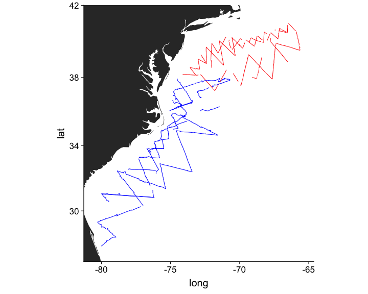<!-- --> --- # Extra information - depth 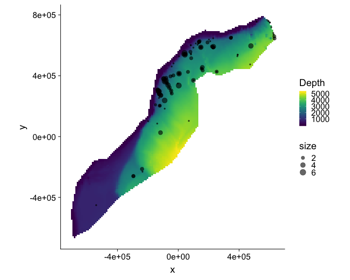<!-- --> --- # Extra information - depth .pull-left[ 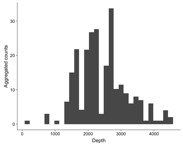<!-- --> ] .pull-right[ - NB this only shows segments where counts > 0 ] --- # Extra information - SST 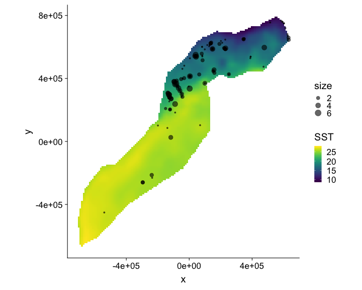<!-- --> --- # Extra information - SST .pull-left[ 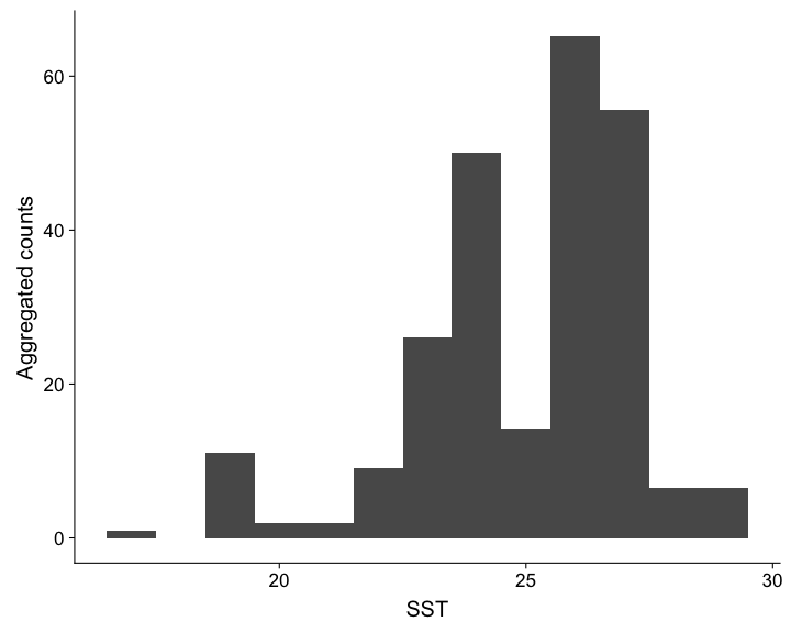<!-- --> ] .pull-right[ - (only segments where counts > 0) ] --- class: inverse, middle, center # You should model that --- # Modelling outputs - Abundance and uncertainty - Arbitrary areas - Numeric values - Maps - Extrapolation (with caution!) - Covariate effects - count/sample as function of covars --- # Modelling requirements - Include detectability - Account for effort - Flexible/interpretable effects - Predictions over an arbitrary area --- class: inverse, middle, center # Accounting for effort --- # Effort .pull-left[ <!-- --> ] .pull-right[ - Have transects - Variation in counts and covars along them - Want a sample unit w/ minimal variation - "Segments": chunks of effort ] --- # Chopping up transects <img src="images/dsmproc.png" alt="Physeter catodon by Noah Schlottman" width=80%> [Physeter catodon by Noah Schlottman](http://phylopic.org/image/dc76cbdb-dba5-4d8f-8cf3-809515c30dbd/) --- class: inverse, middle, center # Flexible, interpretable effects --- # Smooth response 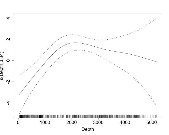<!-- --> --- # Explicit spatial effects 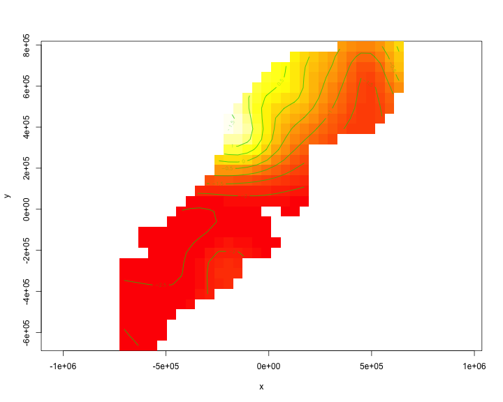<!-- --> --- class: inverse, middle, center # Predictions --- # Predictions over an arbitrary area .pull-left[ 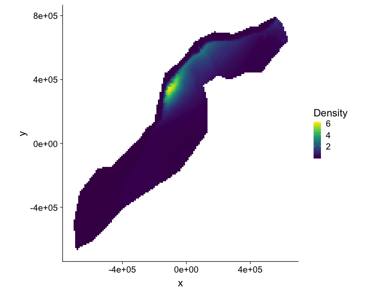<!-- --> ] .pull-right[ - Don't want to be restricted to predict on segments - Predict within survey area - Extrapolate outside (with caution) - Working on a grid of cells ] --- class: inverse, middle, center # Detection information --- # Including detection information - Two options: - adjust areas to account for **effective effort** - use **Horvitz-Thompson estimates** as response --- # Effective effort - Area of each segment, `\(A_j\)` - use `\(A_j\hat{p}_j\)` - think effective strip width ( `\(\hat{\mu} = w\hat{p}\)` ) - Response is counts per segment - "Adjusting for effort" - "Count model" --- # Estimated abundance - Estimate H-T abundance per segment - Effort is area of each segment - "Estimated abundance" per segment $$ \hat{n}_j = \sum_i \frac{s_i}{\hat{p}_i} $$ (where the `\(i\)` observations are in segment `\(j\)`) --- # Detectability and covariates - 2 covariate "levels" in detection function - "Observer"/"observation" -- change **within** segment - "Segment" -- change **between** segments - "Count model" only lets us use segment-level covariates - "Estimated abundance" lets us use either --- # When to use each approach? - Generally "nicer" to adjust effort - Keep response (counts) close to what was observed - **Unless** you want observation-level covariates --- # Availability, perception bias and more - `\(\hat{p}\)` is not always simple! - Availability & perception bias somehow enter - We can make explicit models for this - More later in the course --- # DSM flow diagram <img src="images/dsm-flow.png" alt="DSM process flow diagram" width=100%> --- class: inverse, middle, center # Spatial models --- # Abundance as a function of covariates - Two approaches to model abundance - Explicit spatial models - When: good coverage, fixed area - "Habitat" models (no explicit spatial terms) - When: poorer coverage, extrapolation - We'll cover both approaches here --- class: inverse, middle, center # Data requirements --- # What do we need? - Need to "link" data - ✅ Distance data/detection function - ✅ Segment data - ✅ Observation data (segments 🔗 detections) --- class: inverse, middle, center # Example of spatial data in QGIS --- # Recap - Model counts or estimated abundance - The effort is accounted for differently - Flexible models are good - Incorporate detectability - 2 tables + detection function needed