```{r setup, include=FALSE}
# setup
library(knitr)
library(magrittr)
library(viridis)
library(reshape2)
library(animation)
opts_chunk$set(cache=TRUE, echo=FALSE, warning=FALSE, error=FALSE,
message=FALSE, fig.height=8, fig.width=10)
# some useful libraries
library(RColorBrewer)
library(ggplot2)
library(cowplot)
theme_set(theme_cowplot(20))
```
class: title-slide, inverse, center, middle
# Practical advice

---
class: inverse, center, middle
# Real survey data is messy
---
# Distance sampling in the Real World
- We've talked a lot about models
- We've also talked about assumptions
- Our example is relatively well-behaved
- What can we do about all the nasty real world stuff?
---
# Some days...

---
# Aims
- Here we want to cover common questions
- Not definitive answers
- Some guidance on where to look for answers
---
class: inverse, center, middle
# What should my sample size be?
---
# What do we mean by "sample size"?
- Number of animal (groups) recorded
- *detection function*
- Number of segments
- *spatial model*
- Number of segments with observations
- *spatial model*
---
class: inverse, center, middle
# Re-frame
---
# How would we know when we have enough samples?
- We don't
- Heavily context-dependent
- Go back to assumptions
---
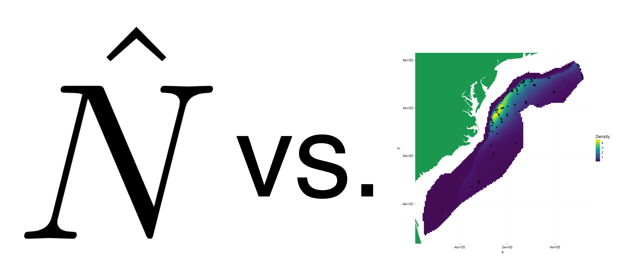
# "How many data?"
```{r df-obs, echo=FALSE, fig.width=15, fig.height=9}
library(Distance)
#set.seed(21)
set.seed(321)
dist1 <- abs(rnorm(30,sd=0.2))
mod1 <- ds(data.frame(distance=dist1, object=1:length(dist1)), adjustment=NULL)
dist2 <- c(abs(rnorm(250,sd=0.02)),
abs(rnorm(750,sd=0.5)))
mod2_full <- ds(data.frame(distance=dist2, object=1:length(dist2)), adjustment=NULL)
mod2_05 <- ds(data.frame(distance=dist2, object=1:length(dist2)), adjustment=NULL, truncation=0.5)
mod2_004 <- ds(data.frame(distance=dist2, object=1:length(dist2)), adjustment=NULL, truncation=0.04)
par(mfrow=c(2,3))
plot(mod1, mainshowpoints=FALSE, pl.den=0)
title(main="n=30", cex.main=5)
plot(1:10, axes=FALSE, type="n", ylab="", xlab="", showpoints=FALSE, pl.den=0)
plot(1:10, axes=FALSE, type="n", ylab="", xlab="", showpoints=FALSE, pl.den=0)
plot(mod2_full, showpoints=FALSE, pl.den=0)
title(main="n=1000", cex.main=5)
plot(mod2_05, showpoints=FALSE, pl.den=0)
title(main="n=747", cex.main=5)
plot(mod2_004, showpoints=FALSE, pl.den=0)
title(main="n=273", cex.main=5)
```
---
# Pilot studies and "you get what you pay for"
- Designing surveys is hard
- Designing surveys is essential
- Better to fail one season than fail for 5, 10 years
- Get information early, get it cheap
- Inform design from a pilot study
---
# Avoiding rules of thumb
- Think about assumptions
- Detection function
- Spatial model
- Think about design
- Spatial coverage
- Covariate coverage
---
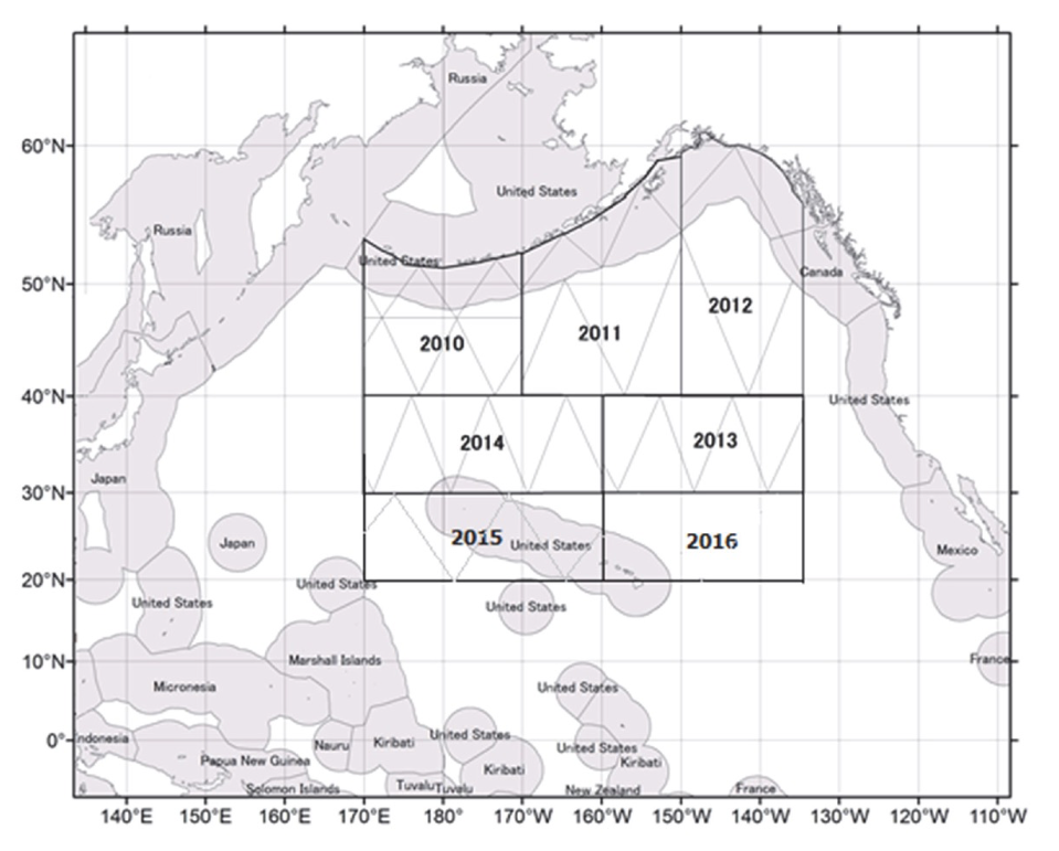
# Spatial coverage (IWC POWER)
 ---
# Covariate coverage
```{r coverage, fig.width=12, echo=FALSE}
library(dsm)
load("../practicals/spermwhale.RData")
df_hr <- ds(dist, truncation=6000, key="hr")
# fit a quick model from previous exericises
dsm_all_tw_rm <- dsm(count~s(x, y, bs="ts") +
s(Depth, bs="ts"),
ddf.obj=df_hr,
segment.data=segs, observation.data=obs,
family=tw(), method="REML")
exclude_fn <- function(top, bottom){
segs2 <- segs[(segs$Depth >0 & segs$Depthtop),]
dsm_a <- dsm(count~s(Depth, bs="ts"),
ddf.obj=df_hr,
segment.data=segs2, observation.data=obs,
family=tw(), method="REML")
plot(dsm_a, scale=0, main=paste0(">",top," and <", bottom), xlim=c(0,5200))
}
par(mfrow=c(1,3), cex.main=2, cex.lab=2, cex.axis=2,
lwd=2, mar=c(5,6,4,2) + 0.1)
exclude_fn(0, Inf)
exclude_fn(3000, 1000)
exclude_fn(5000, 3000)
```
---
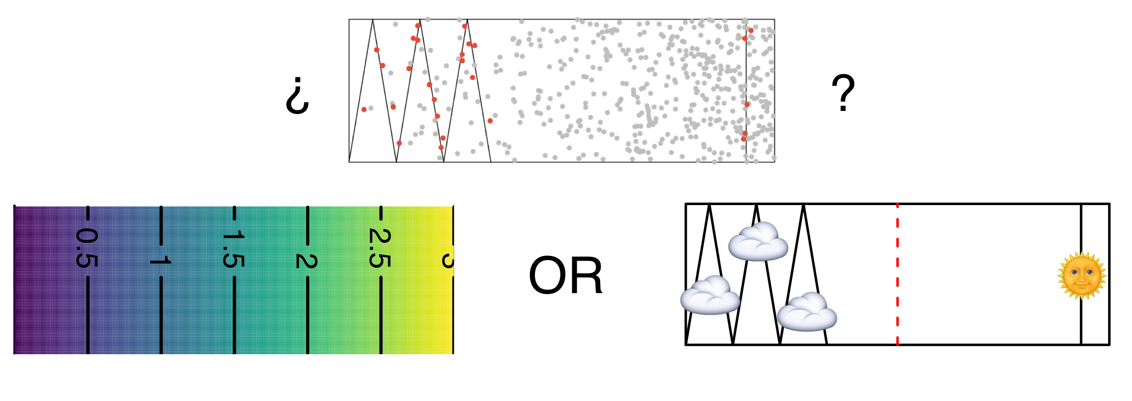
# Sometimes things are complicated
- Weather has a big effect on detectability
- Need to record during survey
- Disambiguate between distribution/detectability
- Potential confounding can be BAD
---
# Visibility during POWER 2014
---
# Covariate coverage
```{r coverage, fig.width=12, echo=FALSE}
library(dsm)
load("../practicals/spermwhale.RData")
df_hr <- ds(dist, truncation=6000, key="hr")
# fit a quick model from previous exericises
dsm_all_tw_rm <- dsm(count~s(x, y, bs="ts") +
s(Depth, bs="ts"),
ddf.obj=df_hr,
segment.data=segs, observation.data=obs,
family=tw(), method="REML")
exclude_fn <- function(top, bottom){
segs2 <- segs[(segs$Depth >0 & segs$Depthtop),]
dsm_a <- dsm(count~s(Depth, bs="ts"),
ddf.obj=df_hr,
segment.data=segs2, observation.data=obs,
family=tw(), method="REML")
plot(dsm_a, scale=0, main=paste0(">",top," and <", bottom), xlim=c(0,5200))
}
par(mfrow=c(1,3), cex.main=2, cex.lab=2, cex.axis=2,
lwd=2, mar=c(5,6,4,2) + 0.1)
exclude_fn(0, Inf)
exclude_fn(3000, 1000)
exclude_fn(5000, 3000)
```
---
# Sometimes things are complicated
- Weather has a big effect on detectability
- Need to record during survey
- Disambiguate between distribution/detectability
- Potential confounding can be BAD

---
# Visibility during POWER 2014
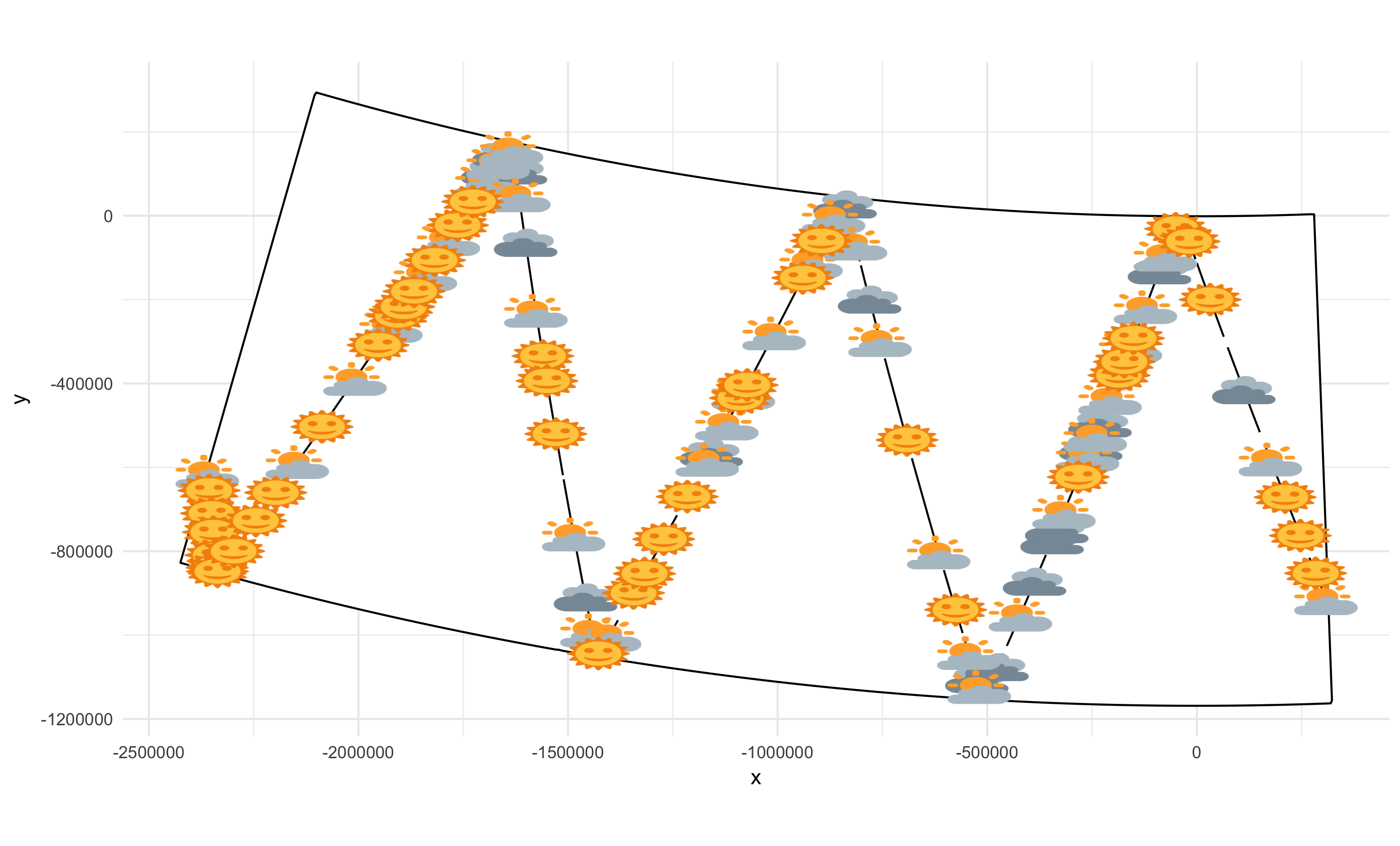 Thanks to Hiroto Murase and co. for this data!
---
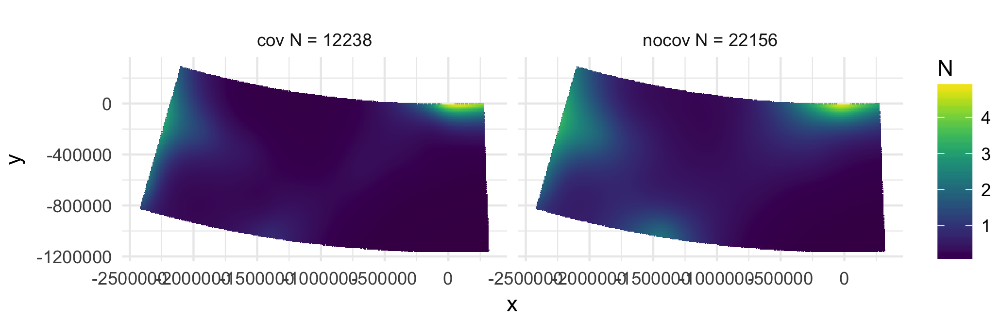
# Covariates can make a big difference!
Thanks to Hiroto Murase and co. for this data!
---
# Covariates can make a big difference!
 ---
# Disappointment
- Sometimes you don't have enough data
- Or, enough coverage
- Or, the right covariates
---
# Disappointment
- Sometimes you don't have enough data
- Or, enough coverage
- Or, the right covariates
Sometimes, you can't build a spatial model
---
class: inverse, center, middle
 [@kitabet](http://twitter.com/kitabet)
---
class: inverse, center, middle
# "Which of options X, Y, Z is correct?"
---
# Alternatives problem
- When faced with options, try them.
- **Where** does the sensitivity lie?
- What's **really** going on?
- What is your **objective**?
---
class: inverse, center, middle
# "How big should our segments be?"
---
# Segment size
- If you think it's an issue test it
- Resolution of covariates also important
- Maybe species-/domain-dependent?
- (Solutions on the horizon to avoid this)
---
class: inverse, center, middle
# "Is our model right?"
---
# Model validation
- Some variety of cross-validation
- Temporal replication
- Leave out 1 year, fit to others, predict, assess
- Spatial "pseudo-jackknife"
- Leave out every $n^{th}$ segment, refit, ...
- (Maybe leave out 2, 3 etc...)
---
class: inverse, center, middle
# Modelling philosophy
---
# Which covariates should we include?
- Dynamic vs static variables
- Spatial terms? Habitat models?
---
class: inverse, center, middle
# Getting help
---
# Resources
- Bibliography has pointers to these topics
- Distance sampling Google Group
- Friendly, helpful, low traffic
- see [distancesampling.org/distancelist.html](http://distancesampling.org/distancelist.html)
---
class: inverse, center, middle
# Advanced topics
---
class: inverse, center, middle
# This is a whirlwind tour...
---
class: inverse, center, middle
# ...and some of this is experimental
---
class: inverse, center, middle
# Smoother zoo
---
# Cyclic smooths
- What if things "wrap around"? (Time, angles, ...)
- Match value and derivative
- Use `bs="cc"`
- See `?smooth.construct.cs.smooth.spec`
[@kitabet](http://twitter.com/kitabet)
---
class: inverse, center, middle
# "Which of options X, Y, Z is correct?"
---
# Alternatives problem
- When faced with options, try them.
- **Where** does the sensitivity lie?
- What's **really** going on?
- What is your **objective**?

---
class: inverse, center, middle
# "How big should our segments be?"
---
# Segment size
- If you think it's an issue test it
- Resolution of covariates also important
- Maybe species-/domain-dependent?
- (Solutions on the horizon to avoid this)
---
class: inverse, center, middle
# "Is our model right?"
---
# Model validation
- Some variety of cross-validation
- Temporal replication
- Leave out 1 year, fit to others, predict, assess
- Spatial "pseudo-jackknife"
- Leave out every $n^{th}$ segment, refit, ...
- (Maybe leave out 2, 3 etc...)
---
class: inverse, center, middle
# Modelling philosophy
---
# Which covariates should we include?
- Dynamic vs static variables
- Spatial terms? Habitat models?
---
class: inverse, center, middle
# Getting help
---
# Resources
- Bibliography has pointers to these topics
- Distance sampling Google Group
- Friendly, helpful, low traffic
- see [distancesampling.org/distancelist.html](http://distancesampling.org/distancelist.html)
---
class: inverse, center, middle
# Advanced topics
---
class: inverse, center, middle
# This is a whirlwind tour...
---
class: inverse, center, middle
# ...and some of this is experimental
---
class: inverse, center, middle
# Smoother zoo
---
# Cyclic smooths
- What if things "wrap around"? (Time, angles, ...)
- Match value and derivative
- Use `bs="cc"`
- See `?smooth.construct.cs.smooth.spec`
 ---
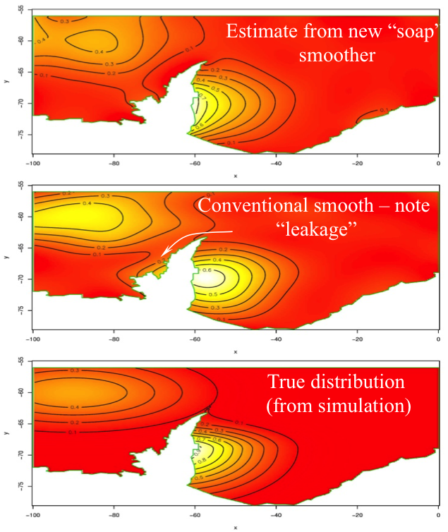
# Smoothing in complex regions
.pull-left[
- Edges are important
- Whales don't live on land
- Bad things happen when we don't account for this
- Include boundary info in smoother
- `?soap`
]
.pull-right[
]
---
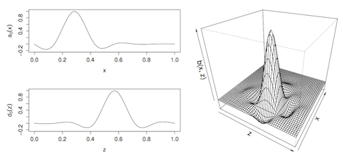
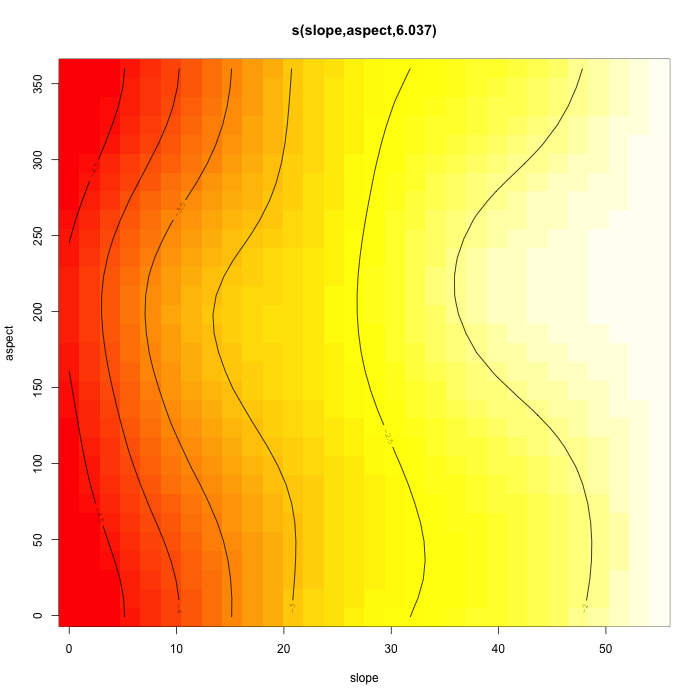
# Multivariate smooths
- Thin plate splines are *isotropic*
- 1 unit in any direction is equal
- Fine for space, not for other things
---
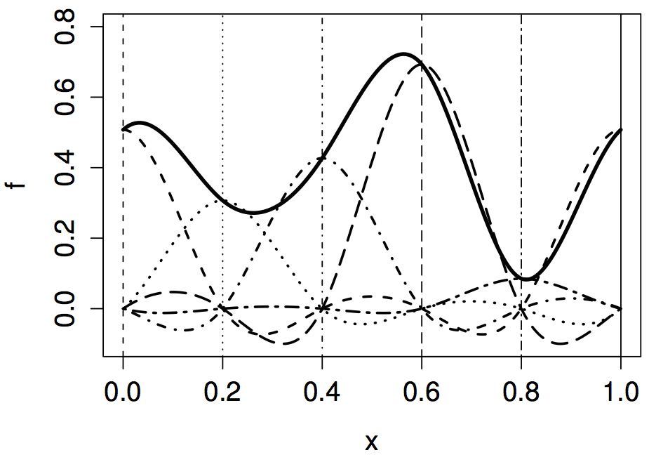
# Tensor products
- $s_{x,z}(x,z) = \sum_{k_1}\sum_{k_2} \beta_k s_x(x)s_z(z)$
- As many covariates as you like! (But takes time)
- `te()` or `ti()` (instead of `s()`)
---
# Black bears like to sunbathe
---
# Smoothing in complex regions
.pull-left[
- Edges are important
- Whales don't live on land
- Bad things happen when we don't account for this
- Include boundary info in smoother
- `?soap`
]
.pull-right[

]
---
# Multivariate smooths
- Thin plate splines are *isotropic*
- 1 unit in any direction is equal
- Fine for space, not for other things
---
# Tensor products
- $s_{x,z}(x,z) = \sum_{k_1}\sum_{k_2} \beta_k s_x(x)s_z(z)$
- As many covariates as you like! (But takes time)
- `te()` or `ti()` (instead of `s()`)

---
# Black bears like to sunbathe
 ---
# Random effects
- normal random effects
- exploits equivalence of random effects and splines `?gam.vcomp`
- useful when you just have a “few” random effects
- `?random.effects`
---
class: inverse, center, middle
# Making things faster
---
# Parallel processing
- Some models are very big/slow
- Run on multiple cores
- Use `engine="bam"`!
- Some constraints in what you can do
- Wood, Goude and Shaw (2015)
---
# Summary
- Lots of complicated problems
- Lots of potential solutions
- (see also "other approaches" mini-lecture)
- Need to get simple things right first
- **Trade assumptions for data**
---
# Random effects
- normal random effects
- exploits equivalence of random effects and splines `?gam.vcomp`
- useful when you just have a “few” random effects
- `?random.effects`
---
class: inverse, center, middle
# Making things faster
---
# Parallel processing
- Some models are very big/slow
- Run on multiple cores
- Use `engine="bam"`!
- Some constraints in what you can do
- Wood, Goude and Shaw (2015)
---
# Summary
- Lots of complicated problems
- Lots of potential solutions
- (see also "other approaches" mini-lecture)
- Need to get simple things right first
- **Trade assumptions for data**