class: title-slide, inverse, center, middle # Multivariate smoothing<br/>&<br/>model selection <div style="position: absolute; bottom: 15px; vertical-align: center; left: 10px"> <img src="images/02-foundation-vertical-white.png" height="200"> </div> --- # The story so far... - How GAMs work - How to include detection info - Simple spatial-only models - How to check those models --- class: inverse, middle, center # Univariate models are fun, but... --- # Ecology is not univariate - Many variables affect distribution - Want to model the **right** ones - Select between possible models - Smooth term selection - Response distribution - Large literature on model selection --- class: inverse, middle, center # Models with multiple smooths --- # Adding smooths - Already know that `+` is our friend - Can build a big model... ```r dsm_all <- dsm(count~s(x, y) + s(Depth) + s(DistToCAS) + s(SST) + s(EKE) + s(NPP), ddf.obj=df_hr, segment.data=segs, observation.data=obs, family=tw()) ``` --- class: inverse, middle, center # Now we have a huge model, what do we do? --- # Term selection .pull-left[ - Two popular approaches (use `\(p\)`-values) **Stepwise selection** - path dependence **All possible subsets** - computationally expensive (fishing?) ] .pull-right[ <img src="images/gnome.jpg"> ] --- # p-values - Test for *zero effect* of a smooth - They are **approximate** for GAMs (but useful) - Reported in `summary` --- # ``` ## ## Family: Tweedie(p=1.25) ## Link function: log ## ## Formula: ## count ~ s(x, y) + s(Depth) + s(DistToCAS) + s(SST) + s(EKE) + ## s(NPP) + offset(off.set) ## ## Parametric coefficients: ## Estimate Std. Error t value Pr(>|t|) ## (Intercept) -20.6369 0.2752 -75 <2e-16 *** ## --- ## Signif. codes: 0 '***' 0.001 '**' 0.01 '*' 0.05 '.' 0.1 ' ' 1 ## ## Approximate significance of smooth terms: ## edf Ref.df F p-value ## s(x,y) 5.236 7.169 1.233 0.2928 ## s(Depth) 3.568 4.439 6.640 1.6e-05 *** ## s(DistToCAS) 1.000 1.000 1.503 0.2205 ## s(SST) 5.927 6.987 2.067 0.0407 * ## s(EKE) 1.763 2.225 2.577 0.0696 . ## s(NPP) 2.393 3.068 0.855 0.4680 ## --- ## Signif. codes: 0 '***' 0.001 '**' 0.01 '*' 0.05 '.' 0.1 ' ' 1 ## ## R-sq.(adj) = 0.224 Deviance explained = 44.9% ## -REML = 368.97 Scale est. = 3.9334 n = 949 ``` --- class: inverse, middle, center # Path dependence is an issue here --- # Term selection during fitting .pull-left[ - Penalty already removes complexity from model - What about using it to remove the whole term? ] .pull-right[  ] --- # Shrinkage approach .pull-left[ - Basis `s(..., bs="ts")` - thin plate splines *with shrinkage* - remove the wiggles **then** remove the "linear" bits - nullspace should be shrunk less than the wiggly part ] .pull-right[  ] --- # Shrinkage example ```r dsm_ts_all <- dsm(count~s(x, y, bs="ts") + s(Depth, bs="ts") + s(DistToCAS, bs="ts") + s(SST, bs="ts") + s(EKE, bs="ts") + s(NPP, bs="ts"), ddf.obj=df_hr, segment.data=segs, observation.data=obs, family=tw()) ``` --- # Model with no shrinkage 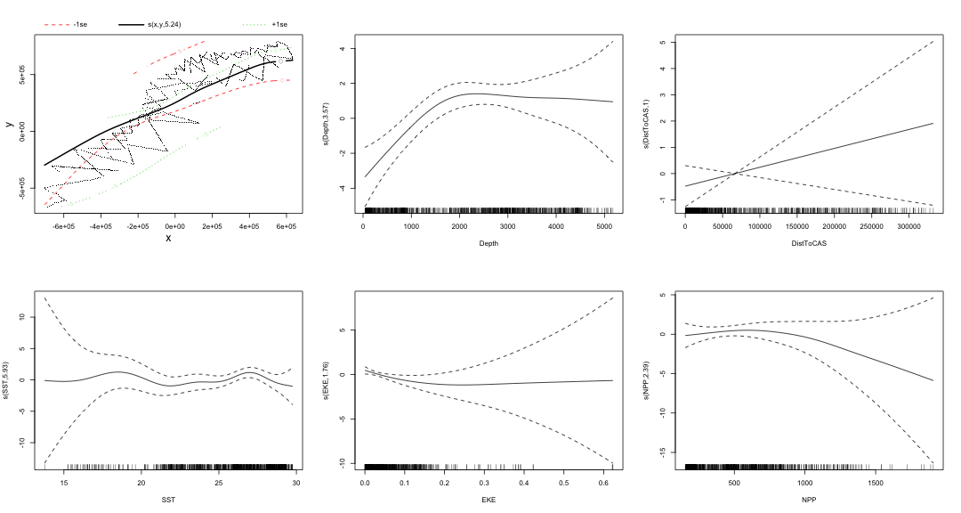<!-- --> --- # ... with shrinkage 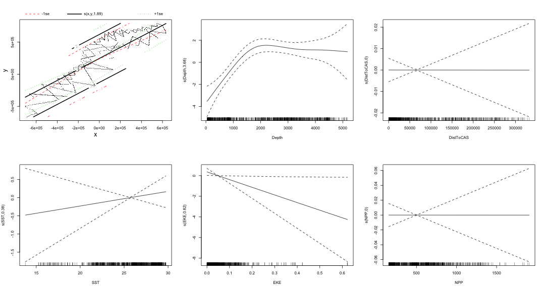<!-- --> --- # ```r summary(dsm_ts_all) ``` ``` ## ## Family: Tweedie(p=1.277) ## Link function: log ## ## Formula: ## count ~ s(x, y, bs = "ts") + s(Depth, bs = "ts") + s(DistToCAS, ## bs = "ts") + s(SST, bs = "ts") + s(EKE, bs = "ts") + s(NPP, ## bs = "ts") + offset(off.set) ## ## Parametric coefficients: ## Estimate Std. Error t value Pr(>|t|) ## (Intercept) -20.260 0.234 -86.59 <2e-16 *** ## --- ## Signif. codes: 0 '***' 0.001 '**' 0.01 '*' 0.05 '.' 0.1 ' ' 1 ## ## Approximate significance of smooth terms: ## edf Ref.df F p-value ## s(x,y) 1.8875209 29 0.705 3.56e-06 *** ## s(Depth) 3.6794182 9 4.811 2.15e-10 *** ## s(DistToCAS) 0.0000934 9 0.000 0.6797 ## s(SST) 0.3826654 9 0.063 0.2160 ## s(EKE) 0.8196256 9 0.499 0.0178 * ## s(NPP) 0.0003570 9 0.000 0.8359 ## --- ## Signif. codes: 0 '***' 0.001 '**' 0.01 '*' 0.05 '.' 0.1 ' ' 1 ## ## R-sq.(adj) = 0.11 Deviance explained = 35.1% ## -REML = 385.04 Scale est. = 4.5486 n = 949 ``` --- # Alternative: extra penalty .pull-left[ - `dsm(..., select=TRUE)` - extra penalty - shrinks everything at the same time - what to shrink "first"? ] .pull-right[  ] --- # Extra penalty example ```r dsm_sel <- dsm(count~s(x, y) + s(Depth) + s(DistToCAS) + s(SST) + s(EKE) + s(NPP), ddf.obj=df_hr, segment.data=segs, observation.data=obs, family=tw(), select=TRUE) ``` --- # ```r summary(dsm_sel) ``` ``` ## ## Family: Tweedie(p=1.266) ## Link function: log ## ## Formula: ## count ~ s(x, y) + s(Depth) + s(DistToCAS) + s(SST) + s(EKE) + ## s(NPP) + offset(off.set) ## ## Parametric coefficients: ## Estimate Std. Error t value Pr(>|t|) ## (Intercept) -20.4285 0.2454 -83.23 <2e-16 *** ## --- ## Signif. codes: 0 '***' 0.001 '**' 0.01 '*' 0.05 '.' 0.1 ' ' 1 ## ## Approximate significance of smooth terms: ## edf Ref.df F p-value ## s(x,y) 7.694e+00 29 1.272 2.67e-07 *** ## s(Depth) 3.645e+00 9 4.005 3.24e-10 *** ## s(DistToCAS) 1.944e-05 9 0.000 0.7038 ## s(SST) 2.010e-04 9 0.000 0.8216 ## s(EKE) 1.417e+00 9 0.630 0.0127 * ## s(NPP) 2.318e-04 9 0.000 0.5152 ## --- ## Signif. codes: 0 '***' 0.001 '**' 0.01 '*' 0.05 '.' 0.1 ' ' 1 ## ## R-sq.(adj) = 0.16 Deviance explained = 40.9% ## -REML = 378 Scale est. = 4.2252 n = 949 ``` --- # Extra penalty example 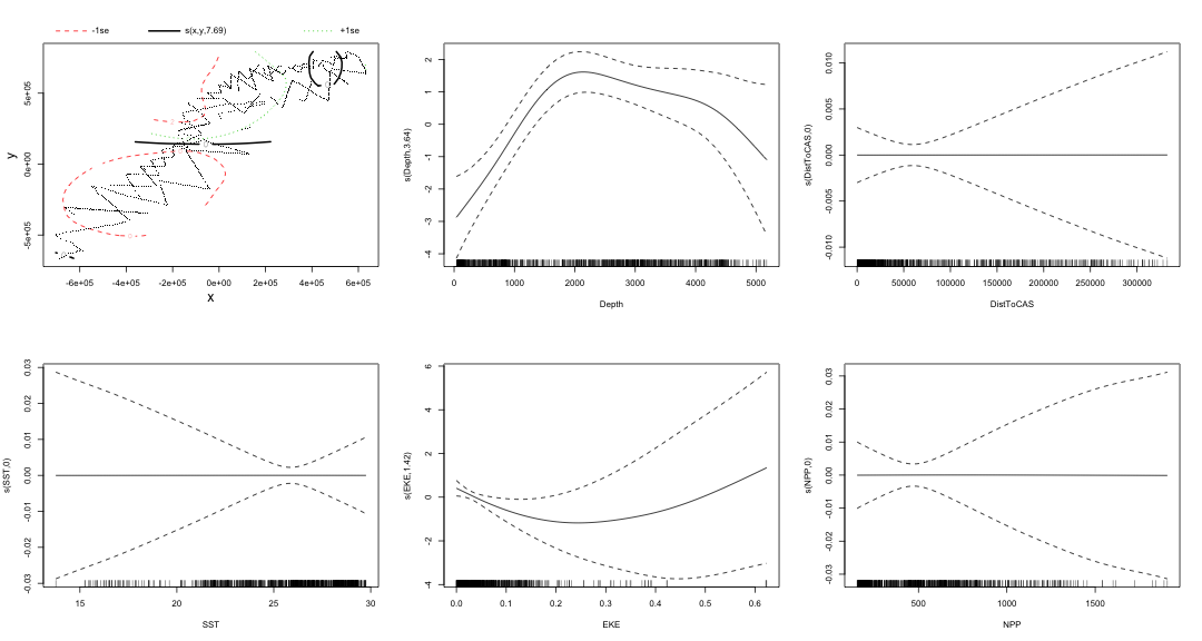<!-- --> --- # EDF comparison <table> <thead> <tr> <th style="text-align:left;"> </th> <th style="text-align:right;"> allterms </th> <th style="text-align:right;"> select </th> <th style="text-align:right;"> ts </th> </tr> </thead> <tbody> <tr> <td style="text-align:left;"> s(x,y) </td> <td style="text-align:right;"> 5.2361 </td> <td style="text-align:right;"> 7.6936 </td> <td style="text-align:right;"> 1.8875 </td> </tr> <tr> <td style="text-align:left;"> s(Depth) </td> <td style="text-align:right;"> 3.5677 </td> <td style="text-align:right;"> 3.6449 </td> <td style="text-align:right;"> 3.6794 </td> </tr> <tr> <td style="text-align:left;"> s(DistToCAS) </td> <td style="text-align:right;"> 1.0001 </td> <td style="text-align:right;"> 0.0000 </td> <td style="text-align:right;"> 0.0001 </td> </tr> <tr> <td style="text-align:left;"> s(SST) </td> <td style="text-align:right;"> 5.9270 </td> <td style="text-align:right;"> 0.0002 </td> <td style="text-align:right;"> 0.3827 </td> </tr> <tr> <td style="text-align:left;"> s(EKE) </td> <td style="text-align:right;"> 1.7628 </td> <td style="text-align:right;"> 1.4174 </td> <td style="text-align:right;"> 0.8196 </td> </tr> <tr> <td style="text-align:left;"> s(NPP) </td> <td style="text-align:right;"> 2.3929 </td> <td style="text-align:right;"> 0.0002 </td> <td style="text-align:right;"> 0.0004 </td> </tr> </tbody> </table> --- # Double penalty can be slow - Lots of smoothing parameters to estimate ```r length(dsm_ts_all$sp) ``` ``` ## [1] 6 ``` ```r length(dsm_sel$sp) ``` ``` ## [1] 12 ``` --- # Removing terms? 1. EDF - Terms with EDF<1 may not be useful (can we remove?) 2. non-significant `\(p\)`-value - Decide on a significance level and use that as a rule (In some sense leaving "shrunk" terms in is more "consistent" in terms of variance estimation, but can be computationally annoying) --- class: inverse, middle, center # Comparing models --- # Comparing models - Usually have >1 option - How can we pick? - Even if we have 1 model, is it any good? --- # Measuring "fit" - Listed in `summary` - Deviance explained - Adjusted `\(R^2\)` (not useful) - Deviance is a generalisation of `\(R^2\)` - Highest likelihood value (*saturated* model) minus estimated model value - (These are usually not very high for DSMs) --- # AIC - Can get AIC from our model - Comparison of AIC fine (but not the end of the story) ```r AIC(dsm_all) ``` ``` ## [1] 1238.307 ``` ```r AIC(dsm_ts_all) ``` ``` ## [1] 1225.822 ``` --- class: inverse, middle, center # Selecting between response distributions --- # Goodness of fit - Q-Q plots - Closer to the line == better 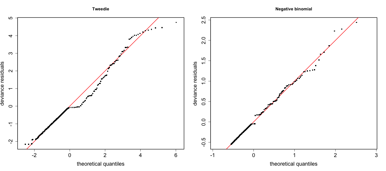<!-- --> --- # Using reference bands ``` qq.gam(dsm_all, asp=1, main="Tweedie", cex=5, rep=100) ``` 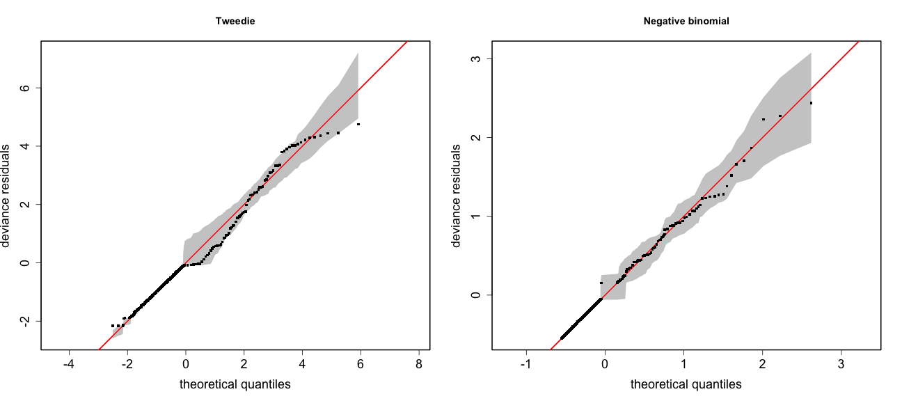<!-- --> --- class: inverse, middle, center # Tobler's first law of geography ## *"Everything is related to everything else, but near things are more related than distant things"* ### Tobler (1970) --- # Implications of Tobler's law 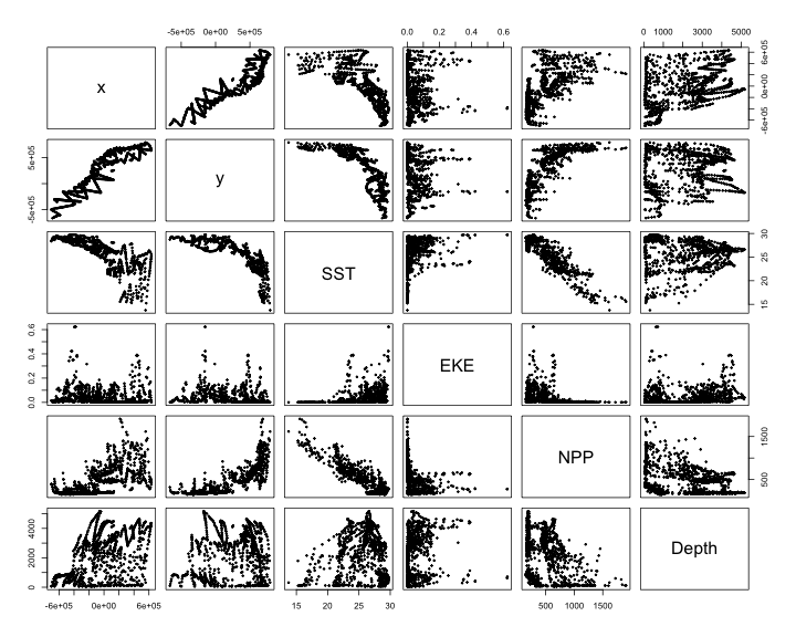<!-- --> --- class: inverse, middle, center ## Covariates are not only correlated (linearly)...<br/><br/>...they are also "concurve" ### *"How much can one smooth be approximated by one or more other smooths?"* --- # Visualising concurvity between terms .pull-left[ 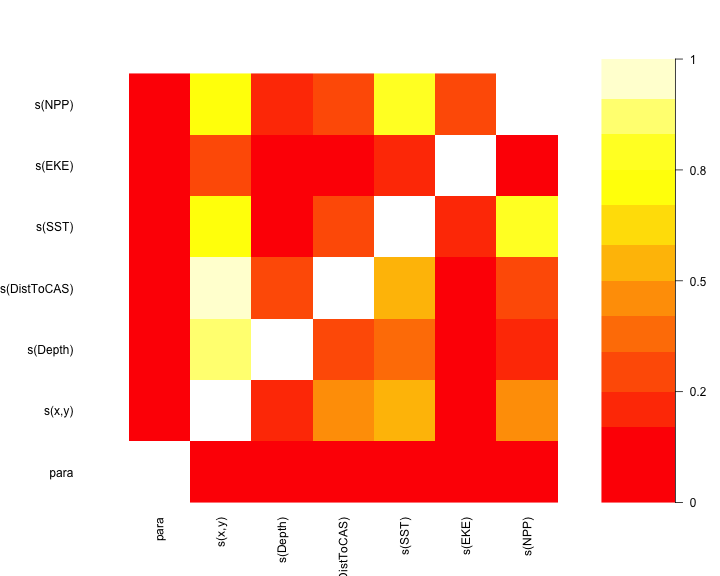<!-- --> ] .pull-right[ - `vis.concurvity` - (Visualisation of `concurvity`) - High values (yellow) = BAD ] --- class: inverse, middle, center # Path dependence --- # Sensitivity - General path dependency? - What if there are highly concurve smooths? - Is the model is sensitive to them? --- # What can we do? - Fit variations excluding smooths - Concurve terms that are excluded early on - Appendix of Winiarski et al (2014) has an example --- # Sensitivity example - `s(Depth)` and `s(x, y)` are highly concurve (0.9067) ``` ## # with depth ``` ``` ## edf Ref.df F p-value ## s(x,y) 1.887521e+00 29 7.053433e-01 3.564239e-06 ## s(Depth) 3.679418e+00 9 4.811277e+00 2.149915e-10 ## s(DistToCAS) 9.339573e-05 9 1.709199e-06 6.796698e-01 ## s(SST) 3.826654e-01 9 6.305406e-02 2.159885e-01 ## s(EKE) 8.196256e-01 9 4.989110e-01 1.775703e-02 ## s(NPP) 3.570476e-04 9 1.615127e-06 8.359159e-01 ``` ``` ## # without depth ``` ``` ## edf Ref.df F p-value ## s(x,y) 1.377758e+01 29 2.588645e+00 1.164871e-12 ## s(DistToCAS) 1.869964e-04 9 2.575100e-06 6.877802e-01 ## s(SST) 3.679648e-04 9 6.186926e-06 6.658640e-01 ## s(EKE) 8.448440e-01 9 5.669750e-01 1.050438e-02 ## s(NPP) 7.993690e-01 9 3.627747e-01 3.229658e-02 ``` --- # Comparison of spatial effects 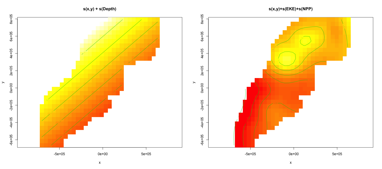<!-- --> --- # Sensitivity example - Refit removing `x` and `y`... ``` ## # without xy ``` ``` ## edf Ref.df F p-value ## s(DistToCAS) 0.0002587354 9 1.804557e-06 8.019754e-01 ## s(SST) 3.7878795045 9 1.401853e+00 2.951200e-03 ## s(Depth) 3.6560507550 9 4.260082e+00 3.020240e-09 ## s(EKE) 0.8089036590 9 4.616991e-01 2.181356e-02 ## s(NPP) 2.4578806949 9 1.371706e+00 1.115487e-03 ``` ``` ## # with xy ``` ``` ## edf Ref.df F p-value ## s(x,y) 1.887521e+00 29 7.053433e-01 3.564239e-06 ## s(Depth) 3.679418e+00 9 4.811277e+00 2.149915e-10 ## s(DistToCAS) 9.339573e-05 9 1.709199e-06 6.796698e-01 ## s(SST) 3.826654e-01 9 6.305406e-02 2.159885e-01 ## s(EKE) 8.196256e-01 9 4.989110e-01 1.775703e-02 ## s(NPP) 3.570476e-04 9 1.615127e-06 8.359159e-01 ``` --- # Comparison of depth smooths 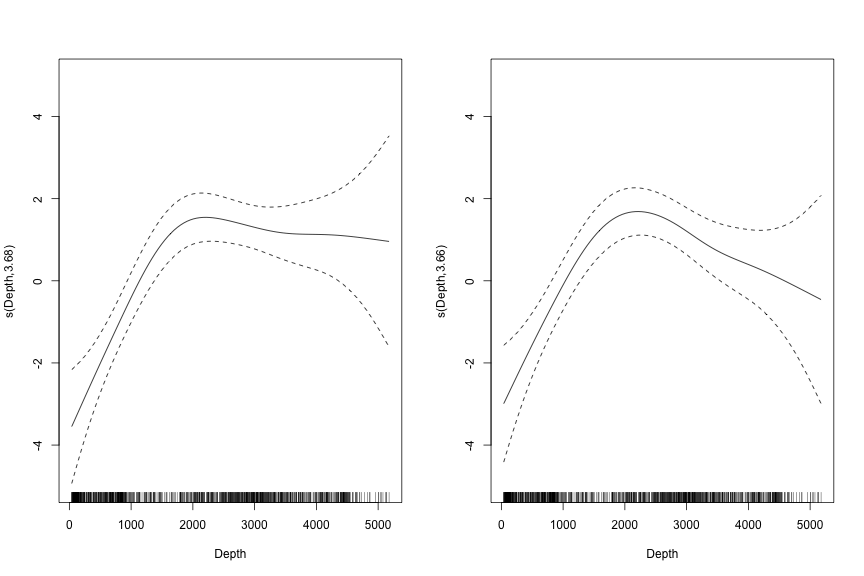<!-- --> --- # Comparing those three models... <table> <thead> <tr> <th style="text-align:left;"> Model </th> <th style="text-align:right;"> AIC </th> <th style="text-align:right;"> Deviance </th> </tr> </thead> <tbody> <tr> <td style="text-align:left;"> `all` </td> <td style="text-align:right;"> 1225.822 </td> <td style="text-align:right;"> 35.10 </td> </tr> <tr> <td style="text-align:left;"> `s(x,y)+s(EKE)+s(NPP)` </td> <td style="text-align:right;"> 1248.172 </td> <td style="text-align:right;"> 34.54 </td> </tr> <tr> <td style="text-align:left;"> `s(SST)+s(Depth)` </td> <td style="text-align:right;"> 1228.106 </td> <td style="text-align:right;"> 39.28 </td> </tr> </tbody> </table> - "Full" model still explains most deviance - We'll come back to this when we do prediction --- class: inverse, middle, center # Recap --- # Recap - Adding smooths - Removing smooths - `\(p\)`-values - shrinkage/extra penalties - Comparing models - Comparing response distributions - Sensitivity