Predictions and variance

# Predictions<br/>and<br/>variance

---

# So far...

- Build, check & select models for detectability
- Build, check & select models for abundance
- Make some ecological inference about smooths
- **What about predictions?**

---

# Let's talk about maps

---

# What does a map mean?

.pull-right[
- Grids!
- Cells are abundance estimate
- "snapshot"
- Sum cells to get abundance
- Sum a subset?
]

---

# Going back to the formula

Count model ( `$j$` observations):

$$
n_j = A_j\hat{p}_j \exp\left[ \beta_0 + s(\text{y}_j) + s(\text{Depth}_j) \right] + \epsilon_j
$$

<br/>
Predictions (index `$r$`):

$$
\hat{n}_r = A_r \exp\left[ \hat{\beta}_0 + \hat{s}(\text{y}_r) + \hat{s}(\text{Depth}_r) \right]
$$

<br/>
Need to "fill-in" values for `$A_r$`, `$\text{y}_r$` and `$\text{Depth}_r$`.

---

# Predicting

- With these values can use `predict` in R
- `predict(model, newdata=data)`

---

# Prediction data

```
##            x      y     Depth    SST      NPP DistToCAS    EKE off.set
## 126 547984.6 788254  153.5983 8.8812 1462.521 11788.974 0.0074   1e+08
## 127 557984.6 788254  552.3107 9.2078 1465.410  5697.248 0.0144   1e+08
## 258 527984.6 778254   96.8199 9.6341 1429.432 13722.626 0.0024   1e+08
## 259 537984.6 778254  138.2376 9.6650 1424.862  9720.671 0.0027   1e+08
## 260 547984.6 778254  505.1439 9.7905 1379.351  8018.690 0.0101   1e+08
## 261 557984.6 778254 1317.5952 9.9523 1348.544  3775.462 0.0193   1e+08
##     LinkID    Nhat_tw
## 126      1 0.01417657
## 127      2 0.05123483
## 258      3 0.01118858
## 259      4 0.01277096
## 260      5 0.04180434
## 261      6 0.45935800
```

---

# A quick word about rasters

- We have talked about rasters a bit
- In R, the `data.frame` is king
- Fortunately `as.data.frame` exists
- Make our "stack" and then convert to `data.frame`

---

# Predictors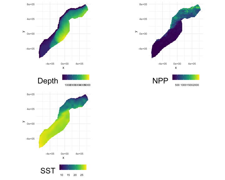

![](dsm5-prediction-variance_files/figure-html/preddata-plot-1.png)

---

# Making a prediction

- Add another column to the prediction data
- Plotting then easier (in R)

```r
predgrid$Nhat_tw <- predict(dsm_all_tw_rm, predgrid)
```

---

# Maps of predictions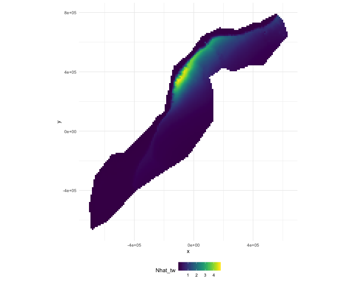

![](dsm5-prediction-variance_files/figure-html/predmap-1.png)
]
.pull-right[

```r
p <- ggplot(predgrid) +
      geom_tile(aes(x=x, y=y,
                    fill=Nhat_tw)) +
      scale_fill_viridis() +
      coord_equal()
print(p)
```
]

---

# Total abundance

Each cell has an abundance, sum to get total

```r
sum(predict(dsm_all_tw_rm, predgrid))
```

```
## [1] 2491.864
```

---

# Subsetting

R subsetting lets you calculate "interesting" estimates:

```r
# how many sperm whales at depths less than 2500m?
sum(predgrid$Nhat_tw[predgrid$Depth < 2500])
```

```
## [1] 1006.272
```

```r
# how many sperm whales East of 0?
sum(predgrid$Nhat_tw[predgrid$x>0])
```

```
## [1] 1383.742
```

---

# Extrapolation

---

# What do we mean by extrapolation?

- Predicting at values outside those observed
- What does "outside" mean?
  - between transects?
  - outside "survey area"?
]
.pull-right[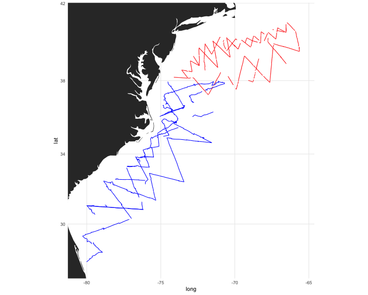

![](dsm5-prediction-variance_files/figure-html/plottracks-1.png)
]

---

# Temporal extrapolation

- Models are temporally implicit (mostly)
- Dynamic variables change seasonally
- Migration can be an issue
- Need to understand what the predictions **are**

---

# Extrapolation

.pull-left[
- Extrapolation is fraught with issues
- Want to be predicting "inside the rug"
- In general, try not to do it!
- (Think about variance too!)
]
.pull-right[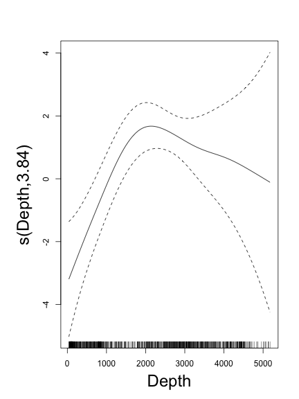
![](dsm5-prediction-variance_files/figure-html/intherug-1.png)
]

---

# Recap

* Using `predict`
* Getting "overall" abundance
* Subsetting
* Plotting in R
* Extrapolation (and its dangers)

---

# Estimating variance

---

# Now we can make predictions

## Now we are dangerous.

---

# Predictions are useless without uncertainty

---

# Where does uncertainty come from?

---

# Sources of uncertainty

- Detection function parameters
- GAM parameters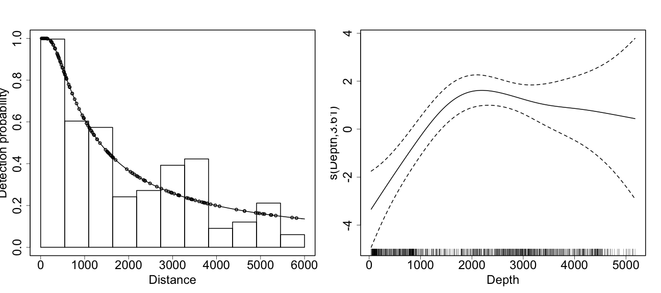

![](dsm5-prediction-variance_files/figure-html/unc-sources-1.png)

---

# GAM + detection function uncertainty

(Getting a little fast-and-loose with the mathematics)

<div style="font-size:150%">
$$
\text{CV}^2\left( \hat{N} \right) \approx \text{CV}^2\left( \text{GAM} \right) +\\
\text{CV}^2\left( \text{detection function}\right)
$$
</div>

---

# Not that simple...

- Assumes detection function and GAM are **independent**
- **Maybe** this is okay?
- (Probably not true?)

---

# Variance propagation

- Include the detectability as term in GAM
- Random effect, mean zero, variance of detection function
- Uncertainty "propagated" through the model
- Paper in bibliography (too much to detail here)
- (Can cover in special topic)

---

# In R...

- Functions in `dsm` to do this
- `dsm.var.gam`
  - assumes spatial model and detection function are independent
- `dsm.var.prop`
  - propagates uncertainty from detection function to spatial model
  - only works for `count` models

---

# Variance of abundance

Using `dsm.var.gam`

```r
dsm_tw_var_ind <- dsm.var.gam(dsm_all_tw_rm, predgrid,
                              off.set=predgrid$off.set)
summary(dsm_tw_var_ind)
```

```
## Summary of uncertainty in a density surface model calculated
##  analytically for GAM, with delta method
## 
## Approximate asymptotic confidence interval:
##     2.5%     Mean    97.5% 
## 1539.018 2491.864 4034.643 
## (Using log-Normal approximation)
## 
## Point estimate                 : 2491.864 
## CV of detection function       : 0.2113123 
## CV from GAM                    : 0.1329 
## Total standard error           : 622.0389 
## Total coefficient of variation : 0.2496
```

---

# Plotting - data processing

- Calculate uncertainty per-cell
- `dsm.var.*` thinks `predgrid` is one "region"
- Need to split data into cells (using `split()`)
- (Could be arbitrary sets of cells, see exercises)
- Need `width` and `height` of cells for plotting

---

# Plotting (code)

```r
predgrid$width <- predgrid$height <- 10*1000
predgrid_split <- split(predgrid, 1:nrow(predgrid))
head(predgrid_split,3)
```

```
## $`1`
##            x      y    Depth    SST      NPP DistToCAS    EKE off.set
## 126 547984.6 788254 153.5983 8.8812 1462.521  11788.97 0.0074   1e+08
##     LinkID    Nhat_tw height width
## 126      1 0.01417657  10000 10000
## 
## $`2`
##            x      y    Depth    SST     NPP DistToCAS    EKE off.set
## 127 557984.6 788254 552.3107 9.2078 1465.41  5697.248 0.0144   1e+08
##     LinkID    Nhat_tw height width
## 127      2 0.05123483  10000 10000
## 
## $`3`
##            x      y   Depth    SST      NPP DistToCAS    EKE off.set
## 258 527984.6 778254 96.8199 9.6341 1429.432  13722.63 0.0024   1e+08
##     LinkID    Nhat_tw height width
## 258      3 0.01118858  10000 10000
```

---

# CV plot

```r
dsm_tw_var_map <- dsm.var.gam(dsm_all_tw_rm, predgrid_split,
                               off.set=predgrid$off.set)
```

.pull-left[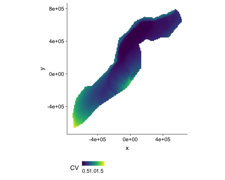
![](dsm5-prediction-variance_files/figure-html/plotit-1.png)
]
.pull-right[
```
p <- plot(dsm_tw_var_map,
          observations=FALSE,
          plot=FALSE) + 
      coord_equal() +
      scale_fill_viridis()
print(p)
```
]

---

# Interpreting CV plots

- Plotting coefficient of variation
- Standardise standard deviation by mean
- `$\text{CV} = \text{se}(\hat{N})/\hat{N}$` (per cell)
- Can be useful to overplot survey effort

---

# Effort overplotted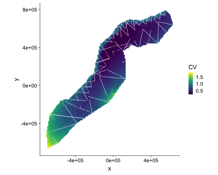

![](dsm5-prediction-variance_files/figure-html/plottracksCV-1.png)

---

# Big CVs

- Here CVs are "well behaved"
- Not always the case (huge CVs possible)
- These can be a pain to plot
- Use `cut()` in R to make categorical variable
  - e.g. `c(seq(0,1, len=10), 2:4, Inf)` or somesuch

---

# Recap

- How does uncertainty arise in a DSM?
- Estimate variance of abundance estimate
- Map coefficient of variation

---

# Let's try that!

---

class: inverse, middle, center
# Extra: brief explanation of uncertainty in smooths

---

# Uncertainty in smooths

- Dashed lines are +/- 2 standard errors
- How do we translate to `$\hat{N}$`?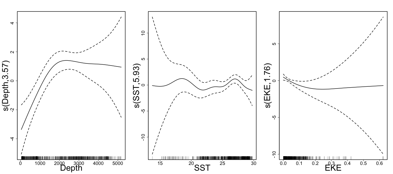

![](dsm5-prediction-variance_files/figure-html/twmod-unc-smooth-1.png)

---

# Back to bases

- Before we expressed smooths as:
  - `$s(x) = \sum_{k=1}^K \beta_k b_k(x)$`
- Theory tells us that:
  - `$\boldsymbol{\beta} \sim N(\boldsymbol{\hat{\beta}}, \mathbf{V}_\boldsymbol{\beta})$`
  - where `$\mathbf{V}_\boldsymbol{\beta}$` is a bit complicated
  - (derived from the smoother matrix)

---

# Predictions to prediction variance (roughly)

- "map" data onto fitted values `$\mathbf{X}\hat{\boldsymbol{\beta}}$`
- "map" prediction matrix to predictions `$\mathbf{X}_p \hat{\boldsymbol{\beta}}$`
- Here `$\mathbf{X}_p$` need to take smooths into account
- pre-/post-multiply by `$\mathbf{X}_p$` to "transform variance"
  - `$\Rightarrow \mathbf{X}_p^\text{T}\mathbf{V}_\boldsymbol{\beta} \mathbf{X}_p$`
  - link scale, need to do another transform for response

---

# Variance propagation

- Refit model with "extra" term

`$\mathbb{E}\left[n_{j}\right]=A_{j}\hat{p}(\boldsymbol{\theta}, z_{j}) \exp\left[ X_{j}\boldsymbol{\beta}+\color{red}{\left.\frac{d\log p\left(\boldsymbol{\theta},z_{j}\right)}{d\boldsymbol{\theta}}\right|_{\boldsymbol{\theta}=\boldsymbol{\theta}_{0}} \boldsymbol{\delta}}\right]$`

- where `$\boldsymbol{\delta}$` is a *random effect*
- fix covariance matrix s.t. `$\boldsymbol{\delta} \sim N(0,-\mathbf{H}^{-1}_\theta)$`
- `$\mathbf{H}_\theta$` is Hessian from detection function