6 Detection function fitting
6.1 Aims
By the end of this practical you should feel confident doing the following:
- Loading data from ArcGIS
.gdbfiles - Working on a
data.framein R to get it into the correct format forDistance - Fitting a detection function using
ds() - Checking detection functions
- Making at goodness of fit plots
- Selecting models using AIC
- Estimating abundance (using R and maths!)
6.2 Preamble
First need to load the requisite R libraries
library(rgdal)
library(ggplot2)
library(Distance)
library(knitr)
6.3 Load the data
The observations are located in a “geodatabase” we created in Arc. We want to pull out the “Sightings” table (called a “layer”) and make it into a data.frame (so it’s easier for R to manipulate).
distdata <- readOGR("Analysis.gdb", layer="Sightings")## OGR data source with driver: OpenFileGDB
## Source: "Analysis.gdb", layer: "Sightings"
## with 137 features
## It has 7 fieldsdistdata <- as.data.frame(distdata)We can check it has the correct format using head:
head(distdata)## Survey GroupSize SeaState Distance SightingTime SegmentID
## 1 en04395 2 3.0 246.0173 2004/06/28 10:22:21 48
## 2 en04395 2 2.5 1632.3934 2004/06/28 13:18:14 50
## 3 en04395 1 3.0 2368.9941 2004/06/28 14:13:34 51
## 4 en04395 1 3.5 244.6977 2004/06/28 15:06:01 52
## 5 en04395 1 4.0 2081.3468 2004/06/29 10:48:31 56
## 6 en04395 1 2.4 1149.2632 2004/06/29 14:35:34 59
## SightingID coords.x1 coords.x2
## 1 1 -65.636 39.576
## 2 2 -65.648 39.746
## 3 3 -65.692 39.843
## 4 4 -65.717 39.967
## 5 5 -65.820 40.279
## 6 6 -65.938 40.612The Distance package expects certain column names to be used. Renaming is much easier to do in R than ArcGIS, so we do it here.
distdata$distance <- distdata$Distance
distdata$object <- distdata$SightingID
distdata$size <- distdata$GroupSize
Let’s see what we did:
head(distdata)## Survey GroupSize SeaState Distance SightingTime SegmentID
## 1 en04395 2 3.0 246.0173 2004/06/28 10:22:21 48
## 2 en04395 2 2.5 1632.3934 2004/06/28 13:18:14 50
## 3 en04395 1 3.0 2368.9941 2004/06/28 14:13:34 51
## 4 en04395 1 3.5 244.6977 2004/06/28 15:06:01 52
## 5 en04395 1 4.0 2081.3468 2004/06/29 10:48:31 56
## 6 en04395 1 2.4 1149.2632 2004/06/29 14:35:34 59
## SightingID coords.x1 coords.x2 distance object size
## 1 1 -65.636 39.576 246.0173 1 2
## 2 2 -65.648 39.746 1632.3934 2 2
## 3 3 -65.692 39.843 2368.9941 3 1
## 4 4 -65.717 39.967 244.6977 4 1
## 5 5 -65.820 40.279 2081.3468 5 1
## 6 6 -65.938 40.612 1149.2632 6 1We now have four “extra” columns.
6.4 Exploratory analysis
Before setting off fitting detection functions, let’s look at the relationship of various variables in the data.
Don’t worry too much about understanding the code that generates these plots at the moment.
6.4.1 Distances
Obviously, the most important covariate in a distance sampling analysis is distance itself. We can plot a histogram of the distances to check that (1) we imported the data correctly and (2) it conforms to the usual shape for line transect data.
hist(distdata$distance, xlab="Distance (m)", main="Distance to sperm whale observations")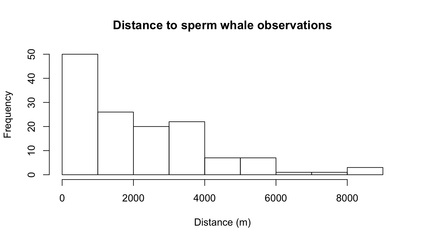
Figure 6.1: Distribution of observed perpendicular detection distances.
6.4.2 Size and distance
We might expect that there will be a relationship between the distance at which we see animals and the size of the groups observed (larger groups are easier to see at larger distances), so let’s plot that to help us visualise the relationship.
# plot of size versus distance and sea state vs distance, linear model and LOESS smoother overlay

# put the data into a simple format, only selecting what we need
distplot <- distdata[,c("distance","size","SeaState")]
names(distplot) <- c("Distance", "Size", "Beaufort")
library(reshape2)
# "melt" the data to have only three columns (try head(distplot))
distplot <- melt(distplot, id.vars="Distance", value.name="covariate")

# make the plot
p <- ggplot(distplot, aes(x=covariate, y=Distance)) +
      geom_point() +
      facet_wrap(~variable, scale="free") +
      geom_smooth(method="loess", se=FALSE) +
      geom_smooth(method="lm", se=FALSE) +
      labs(x="Covariate value", y="Distance (m)")
print(p)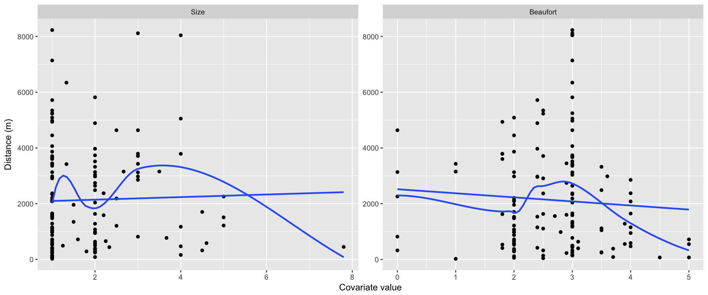
Figure 6.2: Effect of group size upon detection distances.
6.4.3 Distance and sea state
We might also expect that increasing sea state would result in a drop in observations. We can plot histograms of distance for each sea state level (making the sea state take only values 0,1,2,4,5 for this).
distdata$SeaStateCut <- cut(distdata$SeaState,seq(0,5,by=1), include.lowest=TRUE)
p <- ggplot(distdata) +
      geom_histogram(aes(distance)) +
      facet_wrap(~SeaStateCut) +
      labs(x="Distance (m)", y="Count")
print(p)
## `stat_bin()` using `bins = 30`. Pick better value with `binwidth`.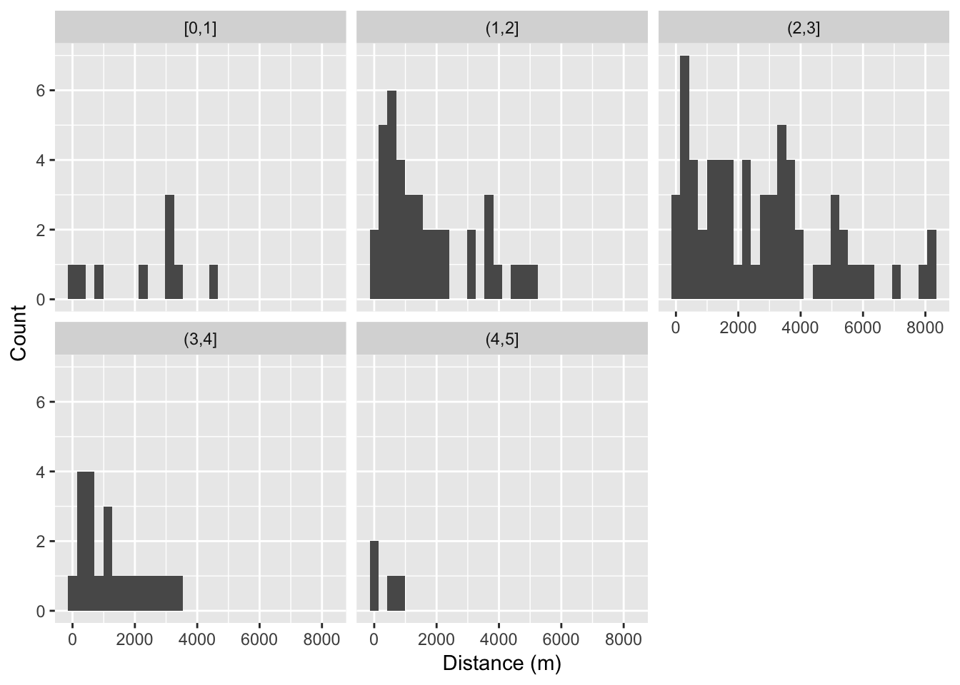
Figure 6.3: Effect of sea state upon detection distances.
6.4.4 Survey effect
Given we are including data from two different surveys we can also investigate the relationship between survey and distances observed.
p <- ggplot(distdata) +
      geom_histogram(aes(distance)) +
      facet_wrap(~Survey) +
      labs(x="Distance (m)", y="Count")
print(p)
## `stat_bin()` using `bins = 30`. Pick better value with `binwidth`.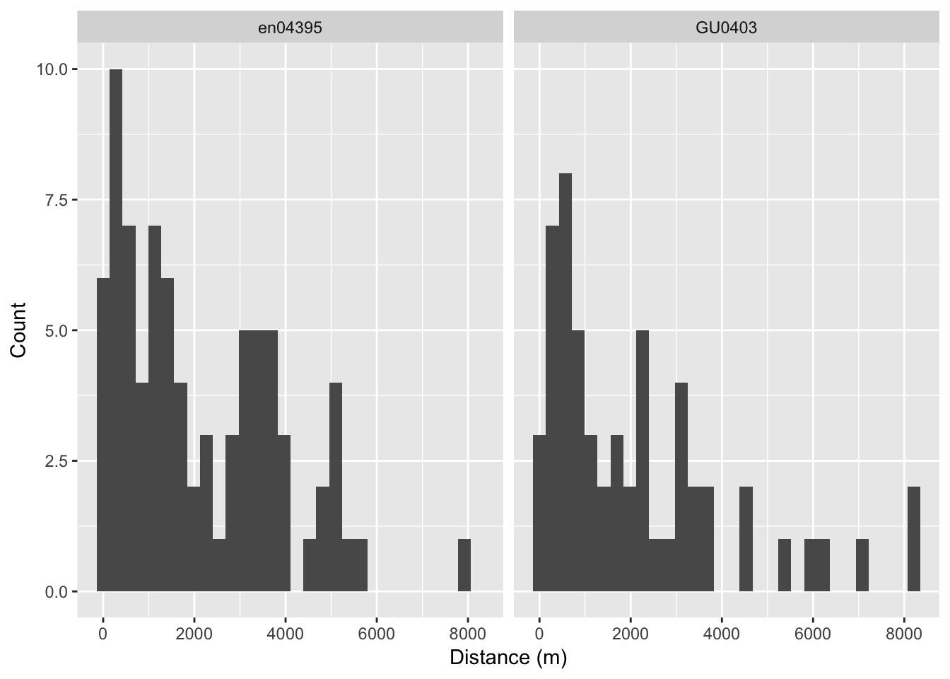
Figure 6.4: Effect of survey upon detection distances.
6.5 Fitting detection functions
It’s now time to fit some detection function models. We’ll use the ds() function from the Distance package to fit the detection function. You can access the help file for the ds() function by typing ?ds – this will give you information about what the different arguments to the function are and what they do.
We can fit a very simple model with the following code:
df_hn <- ds(data=distdata, truncation=6000, key="hn", adjustment=NULL)## Fitting half-normal key function## Key only model: not constraining for monotonicity.## AIC= 2252.06## No survey area information supplied, only estimating detection function.Let’s dissect the call and see what each argument means:
data=distdata: the data to use to fit the model, as we prepared above.truncation=6000: set the truncation distance. Here, observations at distances greater than 6000m will be discarded before fitting the detection function.key="hn": the key function to use for the detection function, in this case half-normal (?dslists the other options).adjustment=NULL: adjustment term series to fit.NULLhere means that no adjustments should be fitted (again?dslists all options).
Other useful arguments for this practical are:
formula=: gives the formula to use for the scale parameter. By default it takes the value~1, meaning the scale parameter is constant and not a function of covariates.order=: specifies the “order” of the adjustments to be used. This is a number (or vector of numbers) specifying the order of the terms. For exampleorder=2fits order 2 adjustments,order=c(2,3)will fit a model with order 2 and 3 adjustments (mathematically, it only makes sense to include order 3 with order 2). By default the value isNULLwhich hasds()select the number of adjustments by AIC.
Distance 7 instructions
Steps to fit detection function using graphical interface-
Distance 7 project has been created for you and can be opened from a .zip archive
- Spend time examining the structure of data in the Data tab.
- Move to the Analysis tab.
- Create a new analysis.
-
Create a data filter to set the truncation distance to 6000m.
-
Create a model specifying MRDS analysis engine with half-normal detection function.
-
Press
Runand examine contents of output window. The results should be identical to those produced in the Summaries section below.
6.5.1 Summaries
We can look at the summary of the fitted detection function using the summary() function:
summary(df_hn)##
## Summary for distance analysis
## Number of observations : 132
## Distance range : 0 - 6000
##
## Model : Half-normal key function
## AIC : 2252.06
##
## Detection function parameters
## Scale coefficient(s):
## estimate se
## (Intercept) 7.900732 0.07884776
##
## Estimate SE CV
## Average p 0.5490484 0.03662569 0.06670757
## N in covered region 240.4159539 21.32287580 0.088691606.5.2 Goodness of fit
Goodness of fit quantile-quantile plot and test results can be accessed using the ddf.gof() function:
ddf.gof(df_hn$ddf)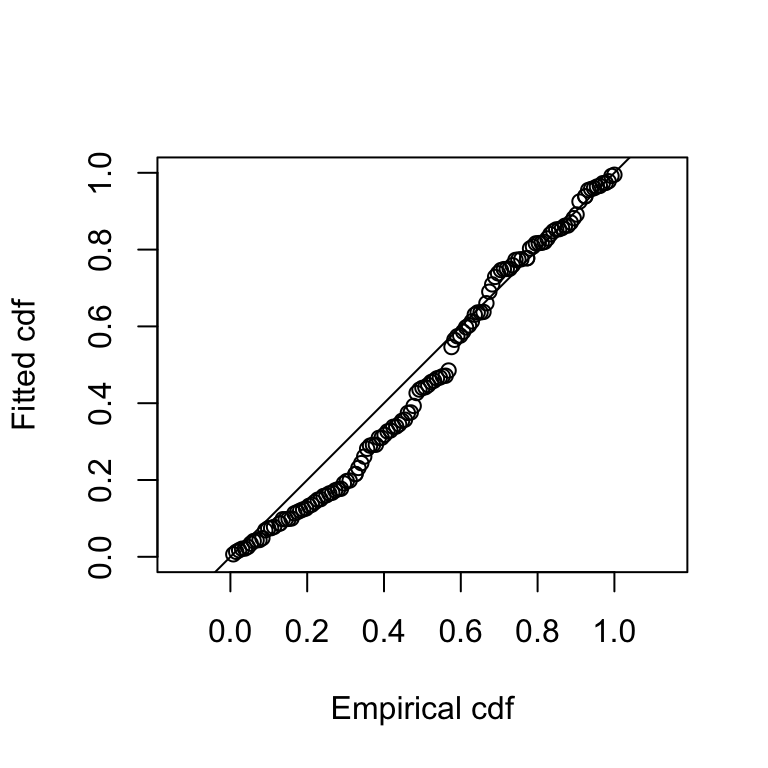
Figure 6.5: Goodness of fit QQ plot of half-normal detection function.
##
## Goodness of fit results for ddf object
##
## Chi-square tests
##             [0,545] (545,1.09e+03] (1.09e+03,1.64e+03] (1.64e+03,2.18e+03]
## Observed  33.000000    20.00000000        19.000000000            8.000000
## Expected  21.708156    20.84245788        19.213254554           17.005089
## Chisquare  5.873634     0.03405238         0.002366986            4.768669
##           (2.18e+03,2.73e+03] (2.73e+03,3.27e+03] (3.27e+03,3.82e+03]
## Observed             9.000000          13.0000000           14.000000
## Expected            14.450499          11.7899695            9.235669
## Chisquare            2.055842           0.1241881            2.457737
##           (3.82e+03,4.36e+03] (4.36e+03,4.91e+03] (4.91e+03,5.45e+03]
## Observed             3.000000           4.0000000            7.000000
## Expected             6.946241           5.0159948            3.477683
## Chisquare            2.241906           0.2057908            3.567525
##           (5.45e+03,6e+03]     Total
## Observed        2.00000000 132.00000
## Expected        2.31498601 132.00000
## Chisquare       0.04285822  21.37457
##
## P = 0.011087 with 9 degrees of freedom
##
## Distance sampling Kolmogorov-Smirnov test
## Test statistic =  0.11192  P =  0.073241
##
## Distance sampling Cramer-von Mises test (unweighted)
## Test statistic =  0.39618  P =  0.073947
Note two things here: 1. We use the $ddf element of the detection function object 2. We’re ignoring the \(\chi^2\) test results, as they rely on binning the distances to calculate test statistics where as Cramer-von Mises and Kolmogorov-Smirnov tests do not.
6.5.3 Plotting
We can plot the models simply using the plot() function:
plot(df_hn)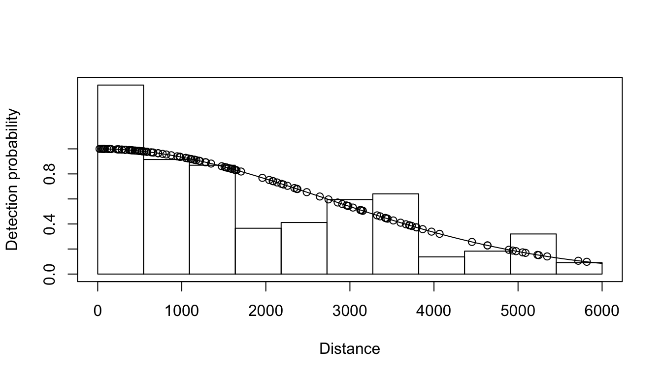
Figure 6.6: Half-normal detection function.
The dots on the plot indicate the distances where observations are. We can remove them (particularly useful for a model without covariates) using the additional argument showpoints=FALSE (try this out!).
6.6 Now you try…
Now try fitting a few models and comparing them using AIC. Don’t try to fit all possible models, just try a selection (say, a hazard-rate, a model with adjustments and a couple with different covariates). You can also try out changing the truncation distance.
Here’s an example to work from. Some tips before you start:
- You can include as many lines as you like in a given chunk (though you may find it more manageable to separate them up, remembering each time to give the chunk a unique name).
- You can run the current line of code in RStudio by hitting
Control+Enter(on Windows/Linux;Command+Enteron Mac). - Giving your models informative names will help later on! Here I’m using
df_to indicate that this is a detection function, then shortened forms of the model form and covariates, separated by underscores, but use what makes sense to you (and future you!).
df_hr_ss_size <- ds(distdata, truncation=6000, adjustment=NULL,
                    key="hr", formula=~SeaState+size)
## Fitting hazard-rate key function## AIC= 2249.327## No survey area information supplied, only estimating detection function.Once you have the hang of writing models and looking at the differences between them, you should move onto the next section.
6.7 Model selection
Looking at the models individually can be a bit unwieldy – it’s nicer to put that data into a table and sort the table by the relevant statistic. The function summarize_ds_models() in the Distance package performs this task for us.
The code below will make a results table with relevant statistics for model selection in it. The summarize_ds_models() function takes a series of object names as its first argument. We can do that with the two models that I fitted like so:
model_table <- summarize_ds_models(df_hn, df_hr_ss_size)
kable(model_table, digits=3, format="latex", booktabs=TRUE, row.names = FALSE, escape=FALSE,
      caption = "Comparison of half normal and hazard rate with sea state and group size.")
(You can add the models you fitted above into this list.)
6.7.0.1 A further note about model selection for the sperm whale data
Note that there is a considerable spike in our distance data. This may be down to observers guarding the trackline (spending too much time searching near zero distance). It’s therefore possible that the hazard-rate model is overfitting to this peak. So we’d like to investigate results from the half-normal model too and see what the effects are on the final spatial models.
6.7.1 Estimating abundance
Just for fun, let’s estimate abundance from these models using a Horvtiz-Thompson-type estimator.
We know the Horvitz-Thompson estimator has the following form: \[ \hat{N} = \frac{A}{a} \sum_{i=1}^n \frac{s_i}{p_i} \] we can calculate each part of this equation in R:
Ais the total area of the region we want to estimate abundance for. This was \(A=5.285e+11 m^2\).ais the total area we surveyed. We know that the total transect length was 9,498,474m and the truncation distance. Knowing that \(a=2wL\) we can calculate \(a\).- \(s_i\) are the group sizes, they are stored in
df_hn$ddf$data$size. - \(p_i\) are the probabilities of detection, we can obtain them using
predict(df_hn$ddf)$fitted.
We know that in general operations are vectorised in R, so calculating c(1, 2, 3)/c(4, 5, 6) will give c(1/4, 2/5, 3/6) so we can just divide the results of getting the \(s_i\) and \(p_i\) values and then use the sum() function to sum them up.
Try out estimating abundance using the formula below using both df_hn and your favourite model from above:
Note that in the solutions to this exercise (posted on the course website) I show how to use the function dht() to estimate abundance (and uncertainty) for a detection function analysis. This involves some more complex data manipulation steps, so we’ve left it out here in favour of getting to grips with the mathematics.
6.7.1.1 Accounting for perception bias
It’s common, especially in marine surveys, for animals at zero distance to be missed by observers. There are several ways to deal with this issue. For now, we are just going to use a very simply constant correction factor to inflate the abundance.
From Palka (2006), we think that observations on the track line were such that \(g(0)=0.46\), we can apply that correction to our abundance estimate (in a very primitive way):
This kind of correction works fine when it’s appropriate to use a single number to adjust by, in general we’d like to model the perception bias, for example using “mark-recapture distance sampling” techniques.
6.7.2 Save model objects
Save your top few models in an RData file, so we can load them up later on. We’ll also save the distance data we used to fit out models.
save(df_hn, df_hr_ss_size, # add you models here, followed by commas!
     distdata,
     file="df-models.RData")
You can check it worked by using the load() function to recover the models.
6.8 References
Palka, D. L. (2006) Summer Abundance Estimates of Cetaceans in US North Atlantic Navy Operating Areas. Northeast Fisheries Science Center Reference Document 06-03