5 Preparing survey data for spatial analysis
5.1 Aims
By the end of this practical, you should feel comfortable:
- Loading data from a geodatabase file into R
- Removing and renaming columns in a
data.frame - Saving data to an
RDatafile
Note we can (and should) re-run this file when we update the Analysis.gdb file to ensure that the data R uses has all of the covariates we want to use in our analysis.
5.2 Preamble
Load some useful packages:
library(rgdal)
library(knitr)
5.3 Load and arrange data
To fit our spatial models we require three objects:
- A detection function.
- The segment data (sometimes called effort data). This tells us how much effort was expended per segment (in this case how far the boat went) and includes the covariates that we want to use to fit our model.
- The observation table. This links the observations in the detection function object to the segments.
In R we can use the rgdal package to access the geodatabase files generated by ArcGIS (R can also access shapefiles and rasters) there are also interfaces to other GIS packages.
It can be useful in general to see which “layers” are available in the geodatabase, for that we can use the ogrListLayers() function:
ogrListLayers("Analysis.gdb")## [1] "EN_Trackline1" "EN_Trackline2" "GU_Trackline2"
## [4] "GU_Sightings" "EN_Sightings" "GU_Trackline"
## [7] "Tracklines" "Tracklines2" "Segments"
## [10] "Sightings" "Segment_Centroids" "Study_Area"
## [13] "US_Atlantic_EEZ"
## attr(,"driver")
## [1] "OpenFileGDB"
## attr(,"nlayers")
## [1] 135.3.1 Segment data
For our analysis the segment data is located in in the “Segment_Centroids” table in the geodatabase. We can import that into R using the readOGR() function:
segs <- readOGR("Analysis.gdb", layer="Segment_Centroids")## OGR data source with driver: OpenFileGDB
## Source: "Analysis.gdb", layer: "Segment_Centroids"
## with 949 features
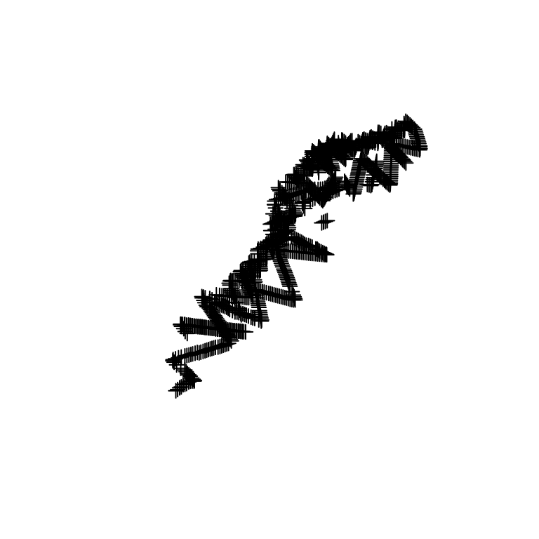
## It has 10 fieldsTo verify we have the right data we can plot it. This will give the locations of each segment:
plot(segs)
Figure 5.1: Segment centroid locations for sperm whale dataset.
A further check would be to use head() to check that the structure of the data is correct. In particular it’s worth checking that the column names are correct and that the number of rows in the data set are correct (dim() will give the number of rows and columns).
It can also be useful to check that the columns are the correct data types. Calling str(segs@data) (or any object loaded using readOGR appended with @data) will reveal the data types of each column. In this case we can see that the CenterTime column has been interpreted as a factor variable rather than as a date/time. We’re not going to use it in our analysis, so we don’t need to worry for now but str() can reveal potential problems with loaded data.
For a deeper look at the values in the data, summary() will give summary statistics for each of the covariates as well as the projection and range of location values (lat/long or in our case x and y). We can compare these with values in ArcGIS.
We can turn the object into a data.frame (so R can better understand it) and then check that it looks like it’s in the right format using head():
segs <- as.data.frame(segs)
head(segs)
## CenterTime SegmentID Length POINT_X POINT_Y Depth
## 1 2004/06/24 07:27:04 1 10288.91 214544.0 689074.3 118.5027
## 2 2004/06/24 08:08:04 2 10288.91 222654.3 682781.0 119.4853
## 3 2004/06/24 09:03:18 3 10288.91 230279.9 675473.3 177.2779
## 4 2004/06/24 09:51:27 4 10288.91 239328.9 666646.3 527.9562
## 5 2004/06/24 10:25:39 5 10288.91 246686.5 659459.2 602.6378
## 6 2004/06/24 11:00:22 6 10288.91 254307.0 652547.2 1094.4402
## DistToCAS SST EKE NPP coords.x1 coords.x2
## 1 14468.1533 15.54390 0.0014442616 1908.129 214544.0 689074.3
## 2 10262.9648 15.88358 0.0014198086 1889.540 222654.3 682781.0
## 3 6900.9829 16.21920 0.0011704842 1842.057 230279.9 675473.3
## 4 1055.4124 16.45468 0.0004101589 1823.942 239328.9 666646.3
## 5 1112.6293 16.62554 0.0002553244 1721.949 246686.5 659459.2
## 6 707.5795 16.83725 0.0006556266 1400.281 254307.0 652547.2As with the distance data, we need to give the columns of the data particular names for them to work with dsm:
segs$x <- segs$POINT_X
segs$y <- segs$POINT_Y
segs$Effort <- segs$Length
segs$Sample.Label <- segs$SegmentID
5.3.2 Observation data
The observation data is exactly what we used to fit out detection function in the previous exercise (though this is not necessarily always true).
obs <- readOGR("Analysis.gdb", layer="Sightings")## OGR data source with driver: OpenFileGDB
## Source: "Analysis.gdb", layer: "Sightings"
## with 137 features
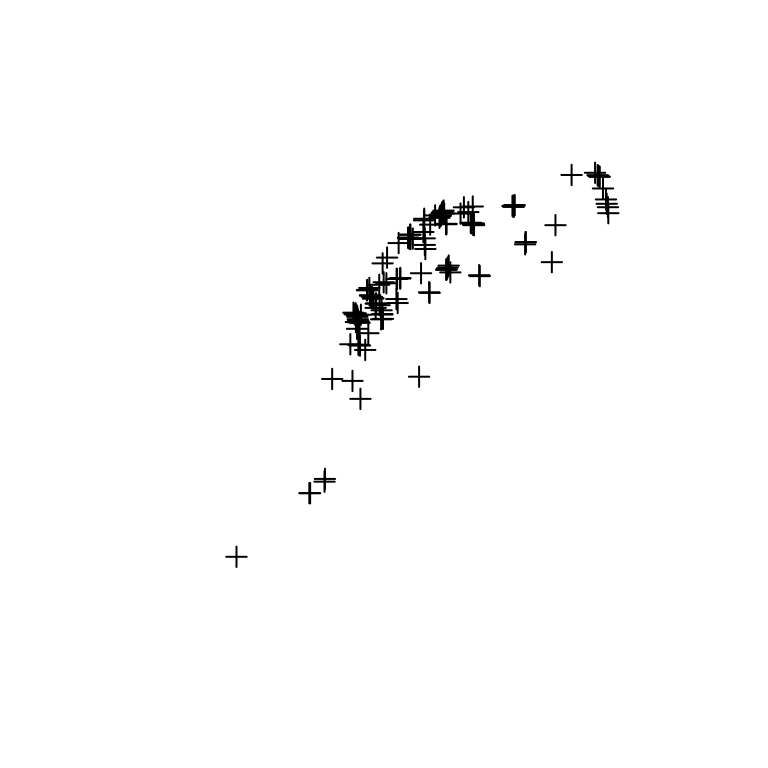
## It has 7 fieldsAgain we can use a plot to see whether the data looks okay. This time we only have the locations of the observations:
plot(obs)
Figure 5.2: Sighting locations for sperm whale dataset.
Again, converting the object to be a data.frame and checking its format using head():
obs <- as.data.frame(obs)
head(obs)
## Survey GroupSize SeaState Distance SightingTime SegmentID
## 1 en04395 2 3.0 246.0173 2004/06/28 10:22:21 48
## 2 en04395 2 2.5 1632.3934 2004/06/28 13:18:14 50
## 3 en04395 1 3.0 2368.9941 2004/06/28 14:13:34 51
## 4 en04395 1 3.5 244.6977 2004/06/28 15:06:01 52
## 5 en04395 1 4.0 2081.3468 2004/06/29 10:48:31 56
## 6 en04395 1 2.4 1149.2632 2004/06/29 14:35:34 59
## SightingID coords.x1 coords.x2
## 1 1 -65.636 39.576
## 2 2 -65.648 39.746
## 3 3 -65.692 39.843
## 4 4 -65.717 39.967
## 5 5 -65.820 40.279
## 6 6 -65.938 40.612Finally, we need to rename some of the columns:
obs$distance <- obs$Distance
obs$object <- obs$SightingID
obs$Sample.Label <- obs$SegmentID
obs$size <- obs$GroupSize
5.4 Save the data
We can now save the data.frames that we’ve created into an RData file so we can use them later.
save(segs, obs, file="sperm-data.RData")