8 Advanced density surface models
8.1 Aims
By the end of this practical, you should feel comfortable:
- Fitting DSMs with multiple smooth terms in them
- Selecting smooth terms by \(p\)-values
- Using shrinkage smoothers
- Selecting between models using deviance, AIC, REML score
- Investigating concurvity in DSMs with multiple smooths
- Investigating sensitivity sensitivity and path dependence
8.2 Load data and packages
library(Distance)
library(dsm)
library(ggplot2)
library(knitr)
library(plyr)
library(reshape2)
Loading the data processed from GIS and the fitted detection function objects from the previous exercises:
load("sperm-data.RData")
load("df-models.RData")
8.3 Exploratory analysis
We can do some exploratory analysis by aggregating the counts to each cell and plotting what’s going on.
Don’t worry about understanding what this code is doing at the moment.
# join the observations onto the segments
join_dat <- join(segs, obs, by="Sample.Label", type="full")
# sum up the observations per segment
n <- ddply(join_dat, .(Sample.Label), summarise, n=sum(size), .drop = FALSE)
# sort the segments by their labsl
segs_eda <- segs[sort(segs$Sample.Label),]
# make a new column for the counts
segs_eda$n <- n$n

# remove the columns we don't need,
segs_eda$CentreTime <- NULL
segs_eda$POINT_X <- NULL
segs_eda$POINT_Y <- NULL
segs_eda$segment.area <- NULL
segs_eda$off.set <- NULL
segs_eda$CenterTime <- NULL
segs_eda$Effort <- NULL
segs_eda$Length <- NULL
segs_eda$SegmentID <- NULL
segs_eda$coords.x1 <- NULL
segs_eda$coords.x2 <- NULL

# "melt" the data so we have four columns:
#   Sample.Label, n (number of observations),
#   variable (which variable), value (its value)
segs_eda <- melt(segs_eda, id.vars=c("Sample.Label", "n"))
# try head(segs_eda)
Finally, we can plot histograms of counts for different values of the covariates:
p <- ggplot(segs_eda) +
       geom_histogram(aes(value, weight=n)) +
       facet_wrap(~variable, scale="free") +
       xlab("Covariate value") +
       ylab("Aggregated counts")
## Warning: Ignoring unknown aesthetics: weightprint(p)## `stat_bin()` using `bins = 30`. Pick better value with `binwidth`.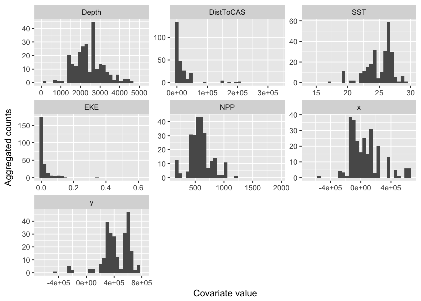
Figure 8.1: Histograms of segment counts at various covariate levels.
We can also just plot the counts against the covariates, note the high number of zeros (but still some interesting patterns):
p <- ggplot(segs_eda) +
       geom_point(aes(value, n)) +
       facet_wrap(~variable, scale="free") +
       xlab("Covariate value") +
       ylab("Aggregated counts")
print(p)
## Warning: Removed 6076 rows containing missing values (geom_point).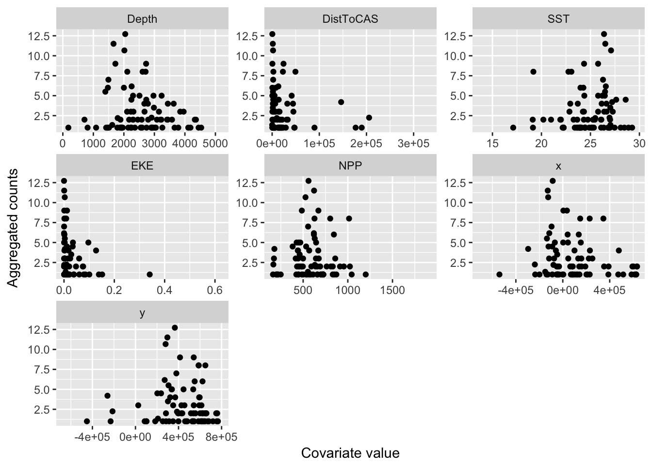
Figure 8.2: Relationship of segment counts to covariate values.
These plots give a very rough idea of the relationships we can expect in the model. Notably these plots don’t take into account interactions between the variables and potential correlations between the terms, as well as detectability.
8.4 Pre-model fitting
As we did in the previous exercise we must remove the observations from the spatial data that we excluded when we fitted the detection function – those observations at distances greater than the truncation.
obs <- obs[obs$distance <= df_hn$ddf$meta.data$width,]Here we’ve used the value of the truncation stored in the detection function object, but we could also use the numeric value (which we can also find by checking the model’s summary()).
Again note that if you want to fit DSMs using detection functions with different truncation distances, then you’ll need to reload the sperm-data.RData and do the truncation again for that detection function.
8.5 Our new friend +
We can build a really big model using + to include all the terms that we want in the model. We can check what’s available to us by using head() to look at the segment table:
head(segs)## CenterTime SegmentID Length POINT_X POINT_Y Depth
## 1 2004/06/24 07:27:04 1 10288.91 214544.0 689074.3 118.5027
## 2 2004/06/24 08:08:04 2 10288.91 222654.3 682781.0 119.4853
## 3 2004/06/24 09:03:18 3 10288.91 230279.9 675473.3 177.2779
## 4 2004/06/24 09:51:27 4 10288.91 239328.9 666646.3 527.9562
## 5 2004/06/24 10:25:39 5 10288.91 246686.5 659459.2 602.6378
## 6 2004/06/24 11:00:22 6 10288.91 254307.0 652547.2 1094.4402
## DistToCAS SST EKE NPP coords.x1 coords.x2 x
## 1 14468.1533 15.54390 0.0014442616 1908.129 214544.0 689074.3 214544.0
## 2 10262.9648 15.88358 0.0014198086 1889.540 222654.3 682781.0 222654.3
## 3 6900.9829 16.21920 0.0011704842 1842.057 230279.9 675473.3 230279.9
## 4 1055.4124 16.45468 0.0004101589 1823.942 239328.9 666646.3 239328.9
## 5 1112.6293 16.62554 0.0002553244 1721.949 246686.5 659459.2 246686.5
## 6 707.5795 16.83725 0.0006556266 1400.281 254307.0 652547.2 254307.0
## y Effort Sample.Label
## 1 689074.3 10288.91 1
## 2 682781.0 10288.91 2
## 3 675473.3 10288.91 3
## 4 666646.3 10288.91 4
## 5 659459.2 10288.91 5
## 6 652547.2 10288.91 6Distance 7 instructions
Fitting complex gams using graphical interface:-
There is nothing difficult about fitting these complex models. The graphical interface is of little help however, you must type the right-hand side of the model you wish to fit into the formula box, just as it is presented in the code snippet below. Much of the formula has scrolled out of the window (but it is there).
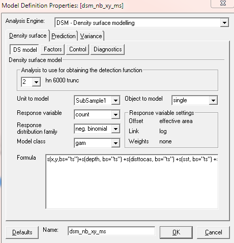
We can then fit a model with the available covariates in it, each as an s() term.
dsm_nb_xy_ms <- dsm(count~s(x,y, bs="ts") +
                       s(Depth, bs="ts") +
                       s(DistToCAS, bs="ts") +
                       s(SST, bs="ts") +
                       s(EKE, bs="ts") +
                       s(NPP, bs="ts"),
                 df_hn, segs, obs,
                 family=nb())
summary(dsm_nb_xy_ms)
##
## Family: Negative Binomial(0.114)
## Link function: log
##
## Formula:
## count ~ s(x, y, bs = "ts") + s(Depth, bs = "ts") + s(DistToCAS,
## bs = "ts") + s(SST, bs = "ts") + s(EKE, bs = "ts") + s(NPP,
## bs = "ts") + offset(off.set)
##
## Parametric coefficients:
## Estimate Std. Error z value Pr(>|z|)
## (Intercept) -20.7732 0.2295 -90.5 <2e-16 ***
## ---
## Signif. codes: 0 '***' 0.001 '**' 0.01 '*' 0.05 '.' 0.1 ' ' 1
##
## Approximate significance of smooth terms:
## edf Ref.df Chi.sq p-value
## s(x,y) 1.8636924 29 19.141 2.90e-05 ***
## s(Depth) 3.4176460 9 46.263 1.65e-11 ***
## s(DistToCAS) 0.0000801 9 0.000 0.9053
## s(SST) 0.0002076 9 0.000 0.5402
## s(EKE) 0.8563344 9 5.172 0.0134 *
## s(NPP) 0.0001018 9 0.000 0.7820
## ---
## Signif. codes: 0 '***' 0.001 '**' 0.01 '*' 0.05 '.' 0.1 ' ' 1
##
## R-sq.(adj) = 0.0947 Deviance explained = 39.2%
## -REML = 382.76 Scale est. = 1 n = 949Notes:
- We’re using
bs="ts"to use the shrinkage thin plate regression spline. More technical detail on these smooths can be found on their manual page?smooth.construct.ts.smooth.spec. - We’ve not specified basis complexity (
k) at the moment. Note that if you want to specify the same complexity for multiple terms, it’s often easier to make a variable that can then be given ask(for example, settingk1<-15and then settingk=k1in the requireds()terms).
8.5.1 Plot
Let’s plot the smooths from this model:
plot(dsm_nb_xy_ms, pages=1, scale=0)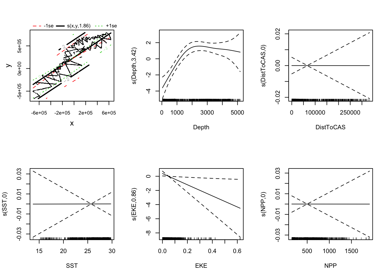
Figure 8.3: Smooths for all covariates with neg-binomial response distribution.
Notes:
- Setting
shade=TRUEgives prettier confidence bands. - As with
vis.gam()the response is on the link scale. scale=0puts each plot on a different \(y\)-axis scale, making it easier to see the effects. Settingscale=-1will put the plots on a common \(y\)-axis scale
We can also plot the bivariate smooth of x and y as we did before, using vis.gam():
vis.gam(dsm_nb_xy_ms, view=c("x","y"), plot.type="contour", too.far=0.1,
        main="s(x,y) (link scale)", asp=1)
Figure 8.4: Fitted surface with all environmental covariates, and neg-binomial response distribution.
Compare this plot to Figure 7.1, generated in the previous practical when only x and y were included in the model.
8.5.2 Check
We can use gam.check() and rqgam.check() to look at the residual check plots for this model.
Do this in the below gaps and comment on the resulting plots and diagnostics.
Looking back through the lecture notes, do you see any problems in these plots or in the text output from gam.check().
You might decide from the diagnostics that you need to increase k for some of the terms in the model. Do this and re-run the above code to ensure that the smooths are flexible enough. The ?choose.k manual page can offer some guidance. Generally if the EDF is close to the value of k you supplied, it’s worth doubling k and refitting to see what happens. You can always switch back to the smaller k if there is little difference.
8.5.3 Select terms
As was covered in the lectures, we can select terms by (approximate) \(p\)-values and by looking for terms that have EDFs significantly less than 1 (those which have been shrunk).
Decide on a significance level that you’ll use to discard terms in the model. Remove the terms that are non-significant at this level and re-run the above checks, summaries and plots to see what happens. It’s helpful to make notes to yourself as you go
It’s easiest to either comment out the terms that are to be removed (using #) or by copying the code chunk above and pasting it below.
Having removed a smooth and reviewed your model, you may decide you wish to remove another. Follow the process again, removing a term, looking at plots and diagnostics.
8.5.4 Compare response distributions
Use the gam.check() to compare quantile-quantile plots between negative binomial and Tweedie distributions for the response.
8.6 Estimated abundance as a response
Again, we’ve only looked at models with count as the response. Try using a detection function with covariates and the abundance.est response in the chunk below:
8.7 Concurvity
Checking concurvity of terms in the model can be accomplished using the concurvity() function.
concurvity(dsm_nb_xy_ms)## para s(x,y) s(Depth) s(DistToCAS) s(SST) s(EKE)
## worst 2.539199e-23 0.9963493 0.9836597 0.9959057 0.9772853 0.7702479
## observed 2.539199e-23 0.8597372 0.8277050 0.9879372 0.9523512 0.6746585
## estimate 2.539199e-23 0.7580838 0.9272203 0.9642030 0.8978412 0.4906765
## s(NPP)
## worst 0.9727752
## observed 0.9525363
## estimate 0.8694619By default the function returns a matrix of a measure of concurvity between one of the terms and the rest of the model.
Compare the output of the models before and after removing terms.
Reading these matrices can be laborious and not very fun. The function vis.concurvity() in the dsm package is used to visualise the concurvity between terms in a model by colour coding the matrix (and blanking out the redundant information).
Again compare the results of plotting for models with different terms.
8.8 Sensitivity
8.8.1 Compare bivariate and additive spatial effects
If we replace the bivariate smooth of location (s(x, y)) with an additive terms (s(x)+s(y)), we may see a difference in the final model (different covariates selected).
dsm_nb_x_y_ms <- dsm(count~s(x, bs="ts") +
                        s(y, bs="ts") +
                        s(Depth, bs="ts") +
                        s(DistToCAS, bs="ts") +
                        s(SST, bs="ts") +
                        s(EKE, bs="ts") +
                        s(NPP, bs="ts"),
                  df_hn, segs, obs,
                  family=nb())
summary(dsm_nb_x_y_ms)
##
## Family: Negative Binomial(0.116)
## Link function: log
##
## Formula:
## count ~ s(x, bs = "ts") + s(y, bs = "ts") + s(Depth, bs = "ts") +
## s(DistToCAS, bs = "ts") + s(SST, bs = "ts") + s(EKE, bs = "ts") +
## s(NPP, bs = "ts") + offset(off.set)
##
## Parametric coefficients:
## Estimate Std. Error z value Pr(>|z|)
## (Intercept) -20.7743 0.2274 -91.37 <2e-16 ***
## ---
## Signif. codes: 0 '***' 0.001 '**' 0.01 '*' 0.05 '.' 0.1 ' ' 1
##
## Approximate significance of smooth terms:
## edf Ref.df Chi.sq p-value
## s(x) 2.875e-01 9 0.337 0.2698
## s(y) 1.709e-05 9 0.000 0.6304
## s(Depth) 3.391e+00 9 37.216 9.88e-10 ***
## s(DistToCAS) 5.393e-04 9 0.000 0.5246
## s(SST) 9.814e-05 9 0.000 0.8176
## s(EKE) 8.670e-01 9 5.582 0.0103 *
## s(NPP) 2.844e+00 9 23.236 9.13e-07 ***
## ---
## Signif. codes: 0 '***' 0.001 '**' 0.01 '*' 0.05 '.' 0.1 ' ' 1
##
## R-sq.(adj) = 0.0993 Deviance explained = 40.7%
## -REML = 383.03 Scale est. = 1 n = 949Try performing model selection as before from this base model and compare the resulting models.
Compare the resulting smooths from like terms in the model. For example, if depth were selected in both models, compare EDFs and plots, e.g.:
par(mfrow=c(1,2))
plot(dsm_nb_xy_ms, select=2)
plot(dsm_nb_x_y_ms, select=3)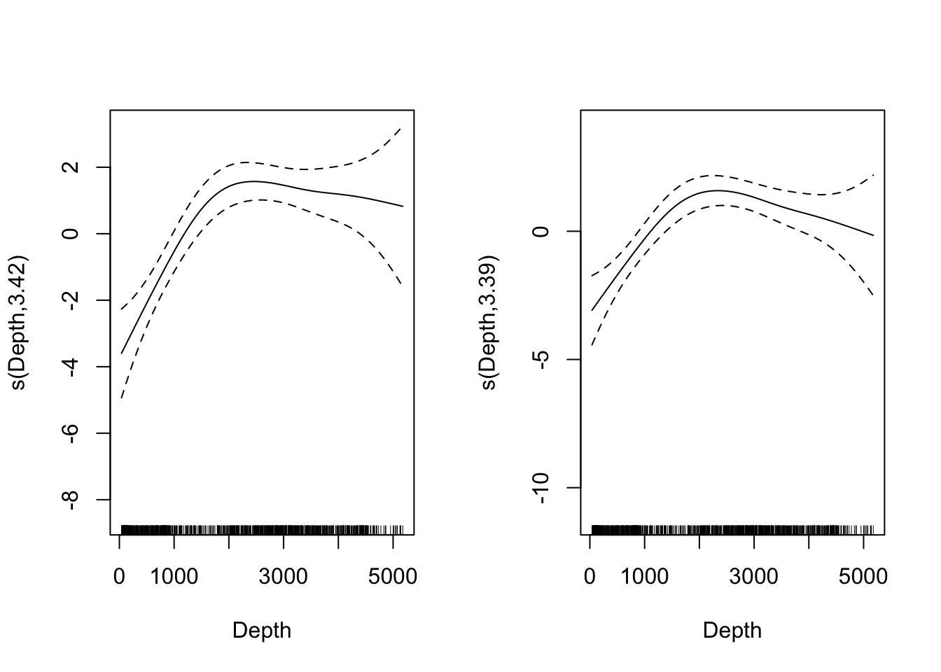
Figure 8.5: Shape of depth covariate response with bivariate s(x,y) and univariate s(x)+s(y).
Note that there select= picks just one term to plot. These are in the order in which the terms occur in the summary() output (so you may well need to adjust the above code).
8.9 Comparing models
As with the detection functions in the earlier exercises, here is a quick function to generate model results tables with appropriate summary statistics:
summarize_dsm <- function(model){

  summ <- summary(model)

  data.frame(response = model$family$family,
             terms    = paste(rownames(summ$s.table), collapse=", "),
             AIC      = AIC(model),
             REML     = model$gcv.ubre,
             "Deviance_explained" = paste0(round(summ$dev.expl*100,2),"%")
            )

}
Distance 7 instructions
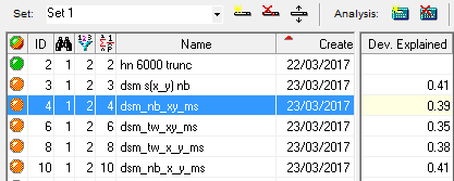
Model comparison using graphical interface:-
The
Results Tableof Distance is good for making model comparisons. There are fewer metrics from which to choose, but metrics in theResults Tablecan be added or removed by using the right-most icon
We can make a list of the models and pass the list to the above function.
# add your models to this list!
model_list <- list(dsm_nb_x_y_ms, dsm_nb_xy_ms)
library(plyr)
summary_table <- ldply(model_list, summarize_dsm)
row.names(summary_table) <- c("dsm_nb_x_y_ms", "dsm_nb_xy_ms")
summary_table <- summary_table[order(summary_table$REML, decreasing=TRUE),]
kable(summary_table,
caption = "Model performance of s(x,y) and s(x)+s(y) in presence of other covariates.")| response | terms | AIC | REML | Deviance_explained | |
|---|---|---|---|---|---|
| dsm_nb_x_y_ms | Negative Binomial(0.116) | s(x), s(y), s(Depth), s(DistToCAS), s(SST), s(EKE), s(NPP) | 752.5585 | 383.0326 | 40.73% |
| dsm_nb_xy_ms | Negative Binomial(0.114) | s(x,y), s(Depth), s(DistToCAS), s(SST), s(EKE), s(NPP) | 754.0326 | 382.7591 | 39.2% |
8.10 Saving models
Now save the models that you’d like to use to predict with later. I recommend saving as many models as you can so you can compare their results in the next practical.
# add your models here
save(dsm_nb_xy_ms, dsm_nb_x_y_ms,
     file="dsms.RData")