9 Prediction using fitted density surface models
Now we’ve fitted some models, let’s use the predict functions and the data from GIS to make predictions of abundance.
9.1 Aims
By the end of this practical, you should feel comfortable:
- Loading raster data into R
- Building a
data.frameof prediction covariates - Making a prediction using the
predict()function - Summing the prediction cells to obtain a total abundance for a given area
- Plotting a map of predictions
- Saving predictions to a raster to be used in ArcGIS
9.2 Loading the packages and data
library(knitr)
library(dsm)
library(ggplot2)
# colourblind-friendly colourschemes
library(viridis)
## Loading required package: viridisLite# to load and save raster data
library(raster)##
## Attaching package: 'raster'## The following object is masked from 'package:nlme':
##
## getData# models with only spatial terms
load("dsms-xy.RData")
# models with all covariates
load("dsms.RData")9.3 Loading prediction data
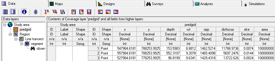
Before we can make predictions we first need to load the covariates into a “stack” from their files on disk using the stack() function from raster. We give stack() a vector of locations to load the rasters from. Note that in RStudio you can use tab-completion for these locations and avoid some typing. At this point we arbitrarily choose the time periods of the SST, NPP and EKE rasters (2 June 2004, or Julian date 153).
predictorStack <- stack(c("Covariates_for_Study_Area/Depth.img",
                          "Covariates_for_Study_Area/GLOB/CMC/CMC0.2deg/analysed_sst/2004/20040602-CMC-L4SSTfnd-GLOB-v02-fv02.0-CMC0.2deg-analysed_sst.img",
                          "Covariates_for_Study_Area/VGPM/Rasters/vgpm.2004153.hdf.gz.img",
                          "Covariates_for_Study_Area/DistToCanyonsAndSeamounts.img",
                          "Covariates_for_Study_Area/Global/DT\ all\ sat/MSLA_ke/2004/MSLA_ke_2004153.img"
                          ))
We need to rename the layers in our stack to match those in the model we are going to use to predict. If you need a refresher on the names that were used there, call summary() on the DSM object.
names(predictorStack) <- c("Depth","SST","NPP", "DistToCAS", "EKE")Now these are loaded, we can coerce the stack into something dsm can talk to using the as.data.frame function. Note we need the xy=TRUE to ensure that x and y are included in the prediction data. We also set the offset value – the area of each cell in our prediction grid.
predgrid <- as.data.frame(predictorStack, xy=TRUE)
predgrid$off.set <- (10*1000)^2
Distance 7 instructions
Access the prediction grid using graphical interface:-
A layer in the Distance project contains georeferenced covariates. Spelling and capitalisation must match variable names used in fitting
dsmmodels. Creation of this prediction grid by importing data can be a labourious process.
We can then predict for the model dsm_nb_xy_ms:
pp <- predict(dsm_nb_xy_ms, predgrid)This is just a list of numbers – the predicted abundance per cell. We can sum these to get the estimated abundance for the study area:
sum(pp, na.rm=TRUE)## [1] 1710.347Because we predicted over the whole raster grid (including those cells without covariate values – e.g. land), some of the values in pp will be NA, so we can ignore them when we sum by setting na.rm=TRUE. We need to do this again when we plot the data too.
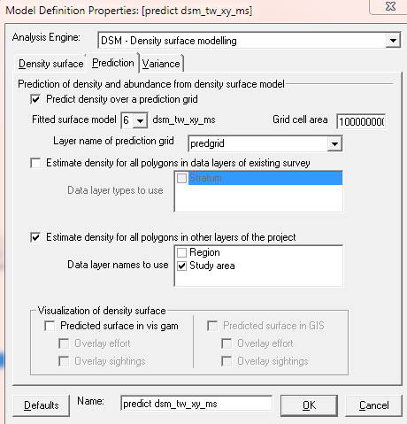
Distance 7 instructions
Prediction to entire study area using graphical interface:-
Using
Predictiontab of DSM model definition, specify density surface model with which to make predictions, size of each cell in the prediction grid (in correct units for the offset), and the layer name of the prediction grid. Tickboxes can be checked for prediction into subregions of the study area and for visualisation.
We can also plot this to get a spatial representation of the predictions:
# assign the predictions to the prediction grid data.frame
predgrid$Nhat_nb_xy <- pp
# remove the NA entries (because of the grid structure of the raster)
predgrid_plot <- predgrid[!is.na(predgrid$Nhat_nb_xy),]
# plot!
p <- ggplot(predgrid_plot) +
      geom_tile(aes(x=x, y=y, fill=Nhat_nb_xy, width=10*1000, height=10*1000)) +
      coord_equal() +
      scale_fill_viridis()
## Warning: Ignoring unknown aesthetics: width, heightprint(p)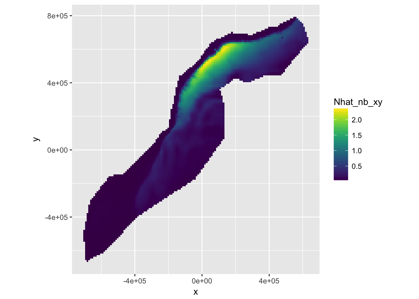
Figure 9.1: Predicted surface for abundance estimates with bivariate spatial smooth along with environmental covariates.
Copy the chunk above and make predictions for the other models you saved in the previous exercises. In particular, compare the models with only spatial terms to those with environmental covariates included.
9.4 Save the prediction to a raster
To be able to load our predictions into ArcGIS, we need to save them as a raster file. First we need to make our predictions into a raster object and save them to the stack we already have:
# setup the storage for the predictions
pp_raster <- raster(predictorStack)
# put the values in, making sure they are numeric first
pp_raster <- setValues(pp_raster, as.numeric(pp))
# name the new, last, layer in the stack
names(pp_raster) <- "Nhat_nb_xy"
We can then save that object to disk as a raster file:
writeRaster(pp_raster, "abundance_raster.img", datatype="FLT4S", overwrite=TRUE)Here we just saved one raster layer: the predictions from model Nhat_nb_xy. Try saving another set of predictions from another model by copying the above chunk.
You can check that the raster was written correctly by using the stack() function, as we did before to load the data and then the plot() function to see what was saved in the raster file.
9.5 Save prediction grid to RData
We’ll need to use the prediction grid and predictor stack again when we calculate uncertainty in the next practical, so let’s save those objects now to save time later.
save(predgrid, predictorStack, file="predgrid.RData")9.6 Extra credit
- Try refitting your models with
family=quasipoisson()as the response distribution. What do you notice about the predicted abundance? - Can you work out a way to use
ldply()from theplyrpackage so that you can usefacet_wrapinggplot2to plot predictions for multiple models in a grid layout?