7 Simple density surface models
7.1 Aims
By the end of this practical, you should feel comfortable:
- Fitting a density surface model using
dsm() - Understanding what the objects that go into a
dsm()call - Understanding the role of the response in the
formula=argument - Understanding the output of
summary()when called on adsmobject - Increasing the
kparameter of smooth terms to increase their flexibility
The example code below uses the df_hn detection function in the density surface models. You can substitute this for your own best model as you go, or copy and paste the code at the end and see what results you get using your model for the detection function.
7.2 Load the packages and data
library(Distance)
library(dsm)
## Loading required package: numDeriv## This is dsm 2.2.15
## Built: R 3.4.1; ; 2017-07-18 14:38:30 UTC; unixlibrary(ggplot2)
library(knitr)Loading the RData files where we saved our results:
load("sperm-data.RData")
load("df-models.RData")
7.3 Pre-model fitting
Before we fit a model using dsm() we must first remove the observations from the spatial data that we excluded when we fitted the detection function – those observations at distances greater than the truncation.
obs <- obs[obs$distance <= df_hn$ddf$meta.data$width, ]Here we’ve used the value of the truncation stored in the detection function object, but we could also use the numeric value (which we can also find by checking the model’s summary()).
Also note that if you want to fit DSMs using detection functions with different truncation distances, then you’ll need to reload the sperm-data.RData and do the truncation again for that detection function.
7.4 Fitting DSMs
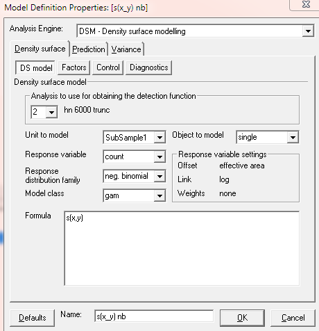
Distance 7 instructions
Steps to fit gams using graphical interface:- Keep the data filter with the truncation distance to 6000m.
-
Set analysis engine to
DSM-Density surface modelling. Specify the response, response distribution, modelling clusters or individuals. Note to specify the analysis number associated with the detection function of interest. In this case the detection function analysis was namedhn 6000 trunc.
-
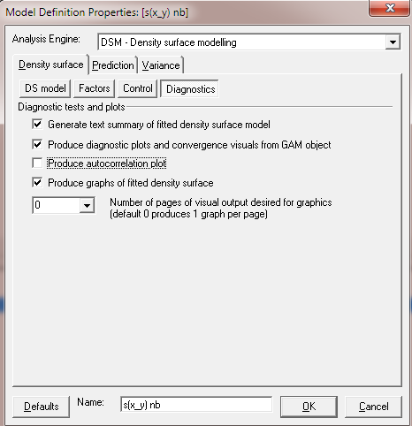
Move to the
Diagnosticsbutton. Tick all boxes except autocorrelation box, which is uninformative for this dataset.
-
Press
Runand examine contents of output window. The results should be identical to those produced in the Summaries section below.
Using the data that we’ve saved so far, we can build a call to the dsm() function and fit out first density surface model. Here we’re only going to look at models that include spatial smooths.
Let’s start with a very simple model – a bivariate smooth of x and y:
dsm_nb_xy <- dsm(count~s(x,y),
                 ddf.obj=df_hn, segment.data = segs, observation.data=obs,
                 family=nb())
Note again that we try to have informative model object names so that we can work out what the main features of the model were from its name alone.
We can look at a summary() of this model. Look through the summary output and try to pick out the important information based on what we’ve talked about in the lectures so far.
summary(dsm_nb_xy)##
## Family: Negative Binomial(0.105)
## Link function: log
##
## Formula:
## count ~ s(x, y) + offset(off.set)
##
## Parametric coefficients:
## Estimate Std. Error z value Pr(>|z|)
## (Intercept) -20.7009 0.2538 -81.56 <2e-16 ***
## ---
## Signif. codes: 0 '***' 0.001 '**' 0.01 '*' 0.05 '.' 0.1 ' ' 1
##
## Approximate significance of smooth terms:
## edf Ref.df Chi.sq p-value
## s(x,y) 17.95 22.23 75.89 6.27e-08 ***
## ---
## Signif. codes: 0 '***' 0.001 '**' 0.01 '*' 0.05 '.' 0.1 ' ' 1
##
## R-sq.(adj) = 0.0879 Deviance explained = 40.7%
## -REML = 392.65 Scale est. = 1 n = 9497.4.1 Visualising output
As discussed in the lectures, the plot output is not terribly useful for bivariate smooths like these. We’ll use vis.gam() to visualise the smooth instead:
vis.gam(dsm_nb_xy, view=c("x","y"), plot.type="contour",
        too.far=0.1, main="s(x,y) (link scale)", asp=1)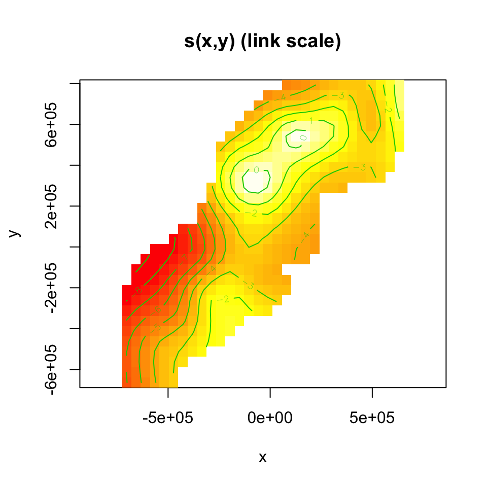
Figure 7.1: Fitted surface (on link scale) for s(x,y)
Notes:
- The plot is on the scale of the link function, the offset is not taken into account – the contour values do not represent abundance, just the “influence” of the smooth.
- We set
view=c("x","y")to display the smooths forxandy(we can choose any two variables in our model to display like this) plot.type="contour"gives this “flat” plot, setplot.type="persp"for a “perspective” plot, in 3D.- The
too.far=0.1argument displays the values of the smooth not “too far” from the data (try changing this value to see what happens). asp=1ensures that the aspect ratio of the plot is 1, making the pixels square.- Read the
?vis.gammanual page for more information on the plotting options.
7.4.2 Setting basis complexity
We can set the basis complexity via the k argument to the s() term in the formula. For example the following re-fits the above model with a much smaller basis complexity than before:
dsm_nb_xy_smallk <- dsm(count~s(x, y, k=10),
                        ddf.obj=df_hn, segment.data = segs,
                        observation.data=obs,
                        family=nb())
Compare the output of vis.gam() for this model to the model with a larger basis complexity.
7.5 Estimated abundance as response
So far we’ve just used count as the response. That is, we adjusted the offset of the model to make it take into account the “effective area” of the segments (see lecture notes for a refresher).
Instead of using count we could use abundance.est, which will leave the segment areas as they are and calculate the Horvitz-Thompson estimates of the abundance per segment and use that as the response in the model. This is most useful when we have covariates in the detection function (though we can use it any time).
Try copying the code that fits the model dsm_nb_xy and make a model dsm_nb_xy_ae that replaces count for abundance.est in the model formula and uses the df_hr_ss_size detection function. Compare the results of summary and plot output between this and the count model.
7.6 Univariate models
Instead of fitting a bivariate smooth of x and y using s(x, y), we could instead use the additive nature and fit the following model:
dsm_nb_x_y <- dsm(count~s(x)+ s(y),
                 ddf.obj=df_hn, segment.data = segs, observation.data=obs,
                 family=nb())
Compare this model with dsm_nb_xy using vis.gam() (Note you can display two plots side-by-side using par(mfrow=c(1,2))). Investigate the output from summary() too, comparing with the other models, adjust k.
7.7 Tweedie response distribution
So far, we’ve used nb() as the response – the negative binomial distribution. We can also try out the Tweedie distribution as a response by replacing nb() with tw().
Try this out and compare the results.
Distance 7 instructions
Changing response or response distribution:- Keep the data filter with the truncation distance to 6000m.
-
Response
countvsabundancecan be specified with pull-down menu. Offsets and link functions (shown on right of window) will change consistent with the response specified.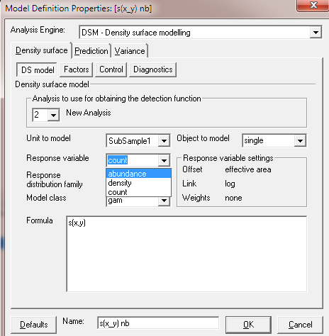
-
Likewise, response distribution family.
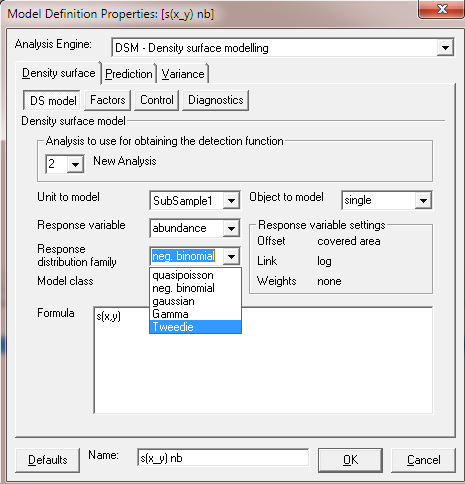
- Be sure you are using the model name field at the bottom of the window to provide detailed name of the models being constructed.
7.8 Save models
It’ll be interesting to see how these models compare to the more complex models we’ll see later on. Let’s save the fitted models at this stage (add your own models to this list so you can use them later).
# add your models here
save(dsm_nb_x_y, dsm_nb_xy,
     file="dsms-xy.RData")
7.9 Extra credit
If you have time, try the following:
- Make the
kvalue very big (~100 or so), what do you notice?